Making full use of the toolbar

When you install Excel, 2 toolbars (standard and formating) will be presented in the application. You should see something like this.


Tool_Bar_Original

The problem with this presentation is that the icons in both toolbars are not fully displayed. In this case, it would have been difficult for you to know all the shortcuts you could use (with the icons) since you can't see them. To make full use of the icons given in these 2 toolbars, you need to separate them. Here is how:

1) Move your mouse cursor along the icons in the toolbars from the left to the right. As you move to the right, the cursor will become a shape with 4 arrows pointing in 4 different directions.



Tool_Bar_Move

2) When the shape appears, click and hold onto the left mouse button and move the tool bar slight downward. The 2 toolbars will be presented in 2 rows and you would be able to see the full range of icons for the 2 toolbars.
3) Let go of the mouse button and you are done. You should be able to see your 2 toolbars presented as follows:


Tool_Bar_Final

Have a blessed weekend.

What is the fastest way to do this?

Happy New Year to you. I wish you and your family a blessed 2006.

My apologies for not updating the blog for such a long time. The last 2 weeks was extremely busy for me as I rush for a number of my projects. I received a query and thought it would be good to share the answer with all of you. The question is as follows:

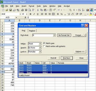
What is the fastest way to do this: check the cells for zero and delete the row if it is zero.

Solution
1) Highlight the list in the Excel Worksheet.
2) Go to Menu and select Edit, Find or use "Ctrl F" (shortcut key)
3) Type in the number "zero"
4) Click on the "Find ALL" button. Make sure that the option exact match is selected. This is to make sure that MS Excel does not return those cells with zero such as 10, 20, 30 , etc.
5.)Select the list by
5a) Go to the first item in the list.
5b) Hold on the shift key and click on the last item in the list.
5c) You have highlighted the entire list (See diagram below)


6) Close the find and replace dialog box.
7) Delete the rows using the following command. Edit >Delete and select entire row and click Ok.

The rows with zeros are deleted.

That's all for today. Drop me an email if this has been useful to you.

Cheers.