Assuming that I have 2 tables. One table contains a list of invoice numbers. Another contains another list of invoice numbers with the second column containing the value of the invoice found in the 1st column.
I try to set up a vlookup formula in the cell next to the invoice number in tbale 1, to look up the invoice number in table 2 based on invoice numerb given in table 1. If the invoice number is found, I want the invoice value (residing in column 2 table 2) to be returned in the cell. In some isntances, the invoice values were returned the right results but on other times, it gives me an error syntax "#N/A". When I check table 2, the invoice number exist but the invoice value was not returned. What could have gone wrong?
To use vlookup to lookup for a particular value/text in another table (Table 2 in this case), you must make sure that the format is the same as that given in Table 1. If the invoice number in Table 1 is a number, while the invoice number in table 2 is a text, vlookup will return a "N/A" results indicating that the invoice number cannot be found. As such, before you use vlookup formula between 2 tables, you must make sure that the format for (the invoice numbers) in table 1 and 2 are the same. Only then can Excel find the value and return the results you are look for.
Monday, February 13, 2006


Tuesday, February 07, 2006
Converting Numbers to Text
You have an Excel worksheet that contains the phone numbers of suppliers and customers. You would like to convert them to text so that you could export these numbers into another IT system. What should you do?
Most users would simply highlight the range of numbers and then format these cells as text. They thought that by doing so, the numbers are all converted to text. THis is not so. When the cells are formated to text, the numbers in these cells remain as numbers. To convert them to text, you need to use the Excel worksheet function called "Text". Assuming that you have a cell in A1 that contains the number 5. To convert it to text, you need to enter the formula =text(A1,"@") , including the "=" into the cell say B1. The number 5 will become a text and when you try to sum up this value with others, it will not included.
Most users would simply highlight the range of numbers and then format these cells as text. They thought that by doing so, the numbers are all converted to text. THis is not so. When the cells are formated to text, the numbers in these cells remain as numbers. To convert them to text, you need to use the Excel worksheet function called "Text". Assuming that you have a cell in A1 that contains the number 5. To convert it to text, you need to enter the formula =text(A1,"@") , including the "=" into the cell say B1. The number 5 will become a text and when you try to sum up this value with others, it will not included.
Tuesday, January 24, 2006
Convert text to number
There are times when you receive a set of records in a worksheet and they are presented in text format. As such you are unable to use these text formatted numbers to perform calculations. In this case, you would need to convert them into numbers.
How then can we convert the text formatted numbers into real numbers that can be used for calculations?
Here is a function that will achieve what you are looking for. It is called the value function. Assuming that you have a text formatted number in A1. To convert it to a number, you just have to type in the formula say in A2 "=value(A1)". The text formatted number would be converted to value and ready for you to perform calculations.
How then can we convert the text formatted numbers into real numbers that can be used for calculations?
Here is a function that will achieve what you are looking for. It is called the value function. Assuming that you have a text formatted number in A1. To convert it to a number, you just have to type in the formula say in A2 "=value(A1)". The text formatted number would be converted to value and ready for you to perform calculations.
Monday, January 16, 2006
Pulling out text from a cell
There are 3 functions that will allow you to pull out text within a cell. These 3 functions will help to pick up certain details that are necessary foranalysis or presentation.
For example, you have a column of text which shows the currency denomination and the amount :
SGD 1000
USD 3203
GBP 342
Yen 543334
In our case, we want to know the denomication of the currency used. To do that, we could use the left function to pull out the first 3 characters in the cell. Assuming that the first cell is in A1, the formula would be written as follows "=left(A1,3)" (exclude the "). By doing so, Excel will pull out the first 3 characters of text from the cell. The results would show SGD, USD, GBP, etc..... RIGHT Function works the same way as LEFT function except that the counting starts from the right.
Mid works in a similar way except that it is capable of pulling out text in middle of a phrase that is in the cell. For example, Cell A1 contains the phrase "Excel contains a lot of advanced function". To pull out the string of text say "contains", you can use the following formula "=mid(A1,7,8)" The formula will pull out the string of text starting from the 7th position and 8 characters from that position.
Have a blessed week ahead.
For example, you have a column of text which shows the currency denomination and the amount :
SGD 1000
USD 3203
GBP 342
Yen 543334
In our case, we want to know the denomication of the currency used. To do that, we could use the left function to pull out the first 3 characters in the cell. Assuming that the first cell is in A1, the formula would be written as follows "=left(A1,3)" (exclude the "). By doing so, Excel will pull out the first 3 characters of text from the cell. The results would show SGD, USD, GBP, etc..... RIGHT Function works the same way as LEFT function except that the counting starts from the right.
Mid works in a similar way except that it is capable of pulling out text in middle of a phrase that is in the cell. For example, Cell A1 contains the phrase "Excel contains a lot of advanced function". To pull out the string of text say "contains", you can use the following formula "=mid(A1,7,8)" The formula will pull out the string of text starting from the 7th position and 8 characters from that position.
Have a blessed week ahead.
Friday, January 06, 2006
Making full use of the toolbar
When you install Excel, 2 toolbars (standard and formating) will be presented in the application. You should see something like this.

Tool_Bar_Original
The problem with this presentation is that the icons in both toolbars are not fully displayed. In this case, it would have been difficult for you to know all the shortcuts you could use (with the icons) since you can't see them. To make full use of the icons given in these 2 toolbars, you need to separate them. Here is how:
1) Move your mouse cursor along the icons in the toolbars from the left to the right. As you move to the right, the cursor will become a shape with 4 arrows pointing in 4 different directions.

Tool_Bar_Move
2) When the shape appears, click and hold onto the left mouse button and move the tool bar slight downward. The 2 toolbars will be presented in 2 rows and you would be able to see the full range of icons for the 2 toolbars.
3) Let go of the mouse button and you are done. You should be able to see your 2 toolbars presented as follows:
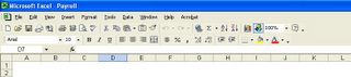
Tool_Bar_Final
Have a blessed weekend.

Tool_Bar_Original

The problem with this presentation is that the icons in both toolbars are not fully displayed. In this case, it would have been difficult for you to know all the shortcuts you could use (with the icons) since you can't see them. To make full use of the icons given in these 2 toolbars, you need to separate them. Here is how:
1) Move your mouse cursor along the icons in the toolbars from the left to the right. As you move to the right, the cursor will become a shape with 4 arrows pointing in 4 different directions.

Tool_Bar_Move
2) When the shape appears, click and hold onto the left mouse button and move the tool bar slight downward. The 2 toolbars will be presented in 2 rows and you would be able to see the full range of icons for the 2 toolbars.
3) Let go of the mouse button and you are done. You should be able to see your 2 toolbars presented as follows:

Tool_Bar_Final
Have a blessed weekend.
Thursday, January 05, 2006
What is the fastest way to do this?
Happy New Year to you. I wish you and your family a blessed 2006.
My apologies for not updating the blog for such a long time. The last 2 weeks was extremely busy for me as I rush for a number of my projects. I received a query and thought it would be good to share the answer with all of you. The question is as follows:
What is the fastest way to do this: check the cells for zero and delete the row if it is zero.
Solution
1) Highlight the list in the Excel Worksheet.
2) Go to Menu and select Edit, Find or use "Ctrl F" (shortcut key)
3) Type in the number "zero"
4) Click on the "Find ALL" button. Make sure that the option exact match is selected. This is to make sure that MS Excel does not return those cells with zero such as 10, 20, 30 , etc.
5.)Select the list by
5a) Go to the first item in the list.
5b) Hold on the shift key and click on the last item in the list.
5c) You have highlighted the entire list (See diagram below)
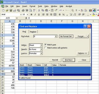
6) Close the find and replace dialog box.
7) Delete the rows using the following command. Edit >Delete and select entire row and click Ok.
The rows with zeros are deleted.
That's all for today. Drop me an email if this has been useful to you.
Cheers.
My apologies for not updating the blog for such a long time. The last 2 weeks was extremely busy for me as I rush for a number of my projects. I received a query and thought it would be good to share the answer with all of you. The question is as follows:
What is the fastest way to do this: check the cells for zero and delete the row if it is zero.
Solution
1) Highlight the list in the Excel Worksheet.
2) Go to Menu and select Edit, Find or use "Ctrl F" (shortcut key)
3) Type in the number "zero"
4) Click on the "Find ALL" button. Make sure that the option exact match is selected. This is to make sure that MS Excel does not return those cells with zero such as 10, 20, 30 , etc.
5.)Select the list by
5a) Go to the first item in the list.
5b) Hold on the shift key and click on the last item in the list.
5c) You have highlighted the entire list (See diagram below)
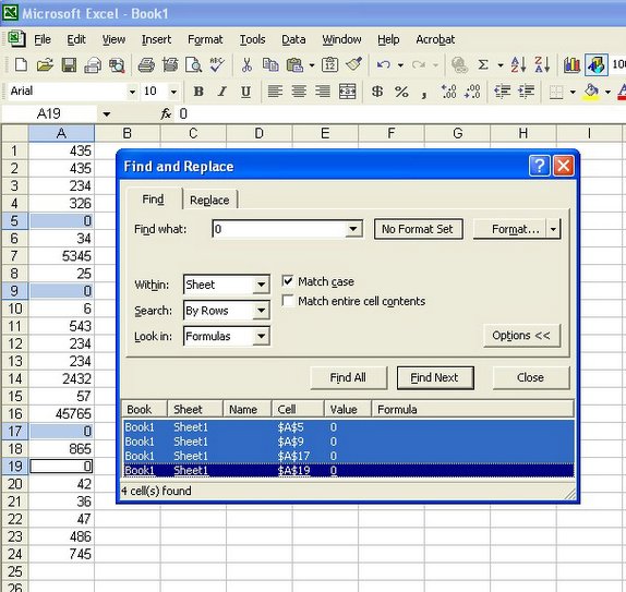
6) Close the find and replace dialog box.
7) Delete the rows using the following command. Edit >Delete and select entire row and click Ok.
The rows with zeros are deleted.
That's all for today. Drop me an email if this has been useful to you.
Cheers.
Friday, December 23, 2005
The Top Ten secrets of Excel
Hi all,
My apologies for not updating the blog for such a long time. I have been overwhelmed with work that I could not find the time to provide new information to you. It is quite coming up with topics out of the blue. As such, I appeal to you to send me some of your Exel-related problems and I will solve it FOC. The condition is that I could share it with others on the blog.
Last week, I have attend a live telecast called the "Learn 10 Secrets About Excel" You can view it online @ https://www118.livemeeting.com/cc/mseventsbmo/viewReg or download the whole e-book at a cheaper.
My apologies for not updating the blog for such a long time. I have been overwhelmed with work that I could not find the time to provide new information to you. It is quite coming up with topics out of the blue. As such, I appeal to you to send me some of your Exel-related problems and I will solve it FOC. The condition is that I could share it with others on the blog.
Last week, I have attend a live telecast called the "Learn 10 Secrets About Excel" You can view it online @ https://www118.livemeeting.com/cc/mseventsbmo/viewReg or download the whole e-book at a cheaper.
Saturday, December 17, 2005
A quick way to copy formula down hundreds of rows.
If you have 2 columns with 1000 rows each (say column A and B) and you created a formula in the first row (e.g. in column C). In most cases, you would have copied the formula throughout the 1000 rows by dragging the formula down. And one problem you faced is that you would take quite a while to drag to the 1000th row. In addition, you are likely to drag beyond the 1000 rows and have to back track.
Now, there is a simpler way. It just take 2 seconds to copy the formula down 1000 rows, or even 10000 rows. What you have to do is to move your mouse cursor to the bottom right corner of the formula cell in column C until a cross appears. Then double click on your left mouse button. Excel will make reference to the cells to the left of the formula cell (Column B in this case) and copy the formula all the way down to the last row (reference to column B). And you are done.
Enjoy your weekend.
Now, there is a simpler way. It just take 2 seconds to copy the formula down 1000 rows, or even 10000 rows. What you have to do is to move your mouse cursor to the bottom right corner of the formula cell in column C until a cross appears. Then double click on your left mouse button. Excel will make reference to the cells to the left of the formula cell (Column B in this case) and copy the formula all the way down to the last row (reference to column B). And you are done.
Enjoy your weekend.
Friday, December 16, 2005
The power of Pivot Table (Part VIII)
My apologies for not blogging for the past 2 days. I have to attend a conference on coporate planning and was busy preparing for my presentation for the conference. I was also trying to meet some project schedules.
I guess this should be the last posting on Pivot Table. There are too many things to cover on Pivot Table that I can spend 2 full days sharing with you all that I know. Having said that, I didn't want to bore you with more details until you have played around with those that I have posted in the last 2 weeks.
Do you know that Excel Pivot Table can give you the raw data that make up a particular result in one single step?
For example, if you are to double click on any one of the Sum of Amount cells, Excel will present the string of records that make up that number in another new worksheet. It will give you all the other details including fields that are not even presented in the pivot table. This is a wonderful function because it allows you to drill down to the most basic details. I don't think crystal report or Business Objects provide that. I may be wrong though.
I guess this should be the last posting on Pivot Table. There are too many things to cover on Pivot Table that I can spend 2 full days sharing with you all that I know. Having said that, I didn't want to bore you with more details until you have played around with those that I have posted in the last 2 weeks.
Do you know that Excel Pivot Table can give you the raw data that make up a particular result in one single step?
For example, if you are to double click on any one of the Sum of Amount cells, Excel will present the string of records that make up that number in another new worksheet. It will give you all the other details including fields that are not even presented in the pivot table. This is a wonderful function because it allows you to drill down to the most basic details. I don't think crystal report or Business Objects provide that. I may be wrong though.
Tuesday, December 13, 2005
The power of Pivot Table (Part VII)
Let's have something simple today. Now if you have a pivot table that shows two attributes on the left column of the pivot table, i.e. Customer Name followed by Promotion as per our pivot table we created in PART V. Do you know that you could hide the details such as those under promotion?
- What you need to do is to double click on a particular customer name and the promotion details are hidden.
- To unhide the details, double click on customer name again and the details under promotion appear.
Saturday, December 10, 2005
The power of Pivot Table (Part VI)
First, let us recap what we have covered so far.
1) We have learnt how to create a pivot table.
2) Format the results
3) Present the company sales results by customers, by promotion and by salesman.
I mentioned in point 3 that the sales results were company's results. What if you want to find out who are the key customers in a particular category or division? Here is how:
a) Move your mouse over the pivot table.
b) Click on the right mouse button and select wizard.
c) When you are brought back to Step 3 of 3 of the wizard, click on the layout button.
d) Notice on the top left hand corner that say page? Drag and drop the field call "division" into the page area.
e) Click Ok to get out of the layout dialog box and click finish to complete the wizard.
f) On the top left hand corner of the pivot table, you will see the field "division". With this, you can select the desired division and the data are filtered to show only the top selling customers by promotion by salesmen for the that division.
I hope I have amazed you with what Excel can do. Please come back if you want to discover more. Do come back if you are still not convinced about the power of Excel.
Have a blessed weekend.
1) We have learnt how to create a pivot table.
2) Format the results
3) Present the company sales results by customers, by promotion and by salesman.
I mentioned in point 3 that the sales results were company's results. What if you want to find out who are the key customers in a particular category or division? Here is how:
a) Move your mouse over the pivot table.
b) Click on the right mouse button and select wizard.
c) When you are brought back to Step 3 of 3 of the wizard, click on the layout button.
d) Notice on the top left hand corner that say page? Drag and drop the field call "division" into the page area.
e) Click Ok to get out of the layout dialog box and click finish to complete the wizard.
f) On the top left hand corner of the pivot table, you will see the field "division". With this, you can select the desired division and the data are filtered to show only the top selling customers by promotion by salesmen for the that division.
I hope I have amazed you with what Excel can do. Please come back if you want to discover more. Do come back if you are still not convinced about the power of Excel.
Have a blessed weekend.
Friday, December 09, 2005
The power of pivot table (Part V)
If you have followed through my recent blogs on The power of Pivot Table Part I to Part VI, you would have formatted the pivot table in a presentable format with the customers ranked by the total amount they have purchased from the company in descending order. The pivot table would have displayed which salesmen have sold products to the customers.
You may find that the above format is not sufficient for you to make decision on how you should classify the customers. You wonder whether the top customers are purchasing more of promotion items or normal items from you. Is pivot table able to do that? The answer is yes and here is how:
1) Move the mouse pointer over the pivot table.
2) Right click the mouse button.
3) A pop up menu will appear. Look for wizard and select it.
4) You are brought back to the step 3 of the pivot table wizard. Click on the layout button.
5) Now drag the field "promotion" from the list to the column area right below the customer name.
6) Click Ok and finished.
7) You should see the field "promotion" appearing on the left side of the "customer name"
8) Move the mouse button over the the right border of the row label as shown in this diagram.
9) Left click on the mouse button.
10) All the sub-total would be selected.
11) Highlight the sub-total with a color. For me, I would choose yellow.
Now you are able to make more informed business decisions with the additional dimension added.
Note: You can add as many dimensions to the column or row area. But remember that having more may not be better. Try not to micro analyse.
Take care and God Bless.
You may find that the above format is not sufficient for you to make decision on how you should classify the customers. You wonder whether the top customers are purchasing more of promotion items or normal items from you. Is pivot table able to do that? The answer is yes and here is how:
1) Move the mouse pointer over the pivot table.
2) Right click the mouse button.
3) A pop up menu will appear. Look for wizard and select it.
4) You are brought back to the step 3 of the pivot table wizard. Click on the layout button.
5) Now drag the field "promotion" from the list to the column area right below the customer name.
6) Click Ok and finished.
7) You should see the field "promotion" appearing on the left side of the "customer name"
8) Move the mouse button over the the right border of the row label as shown in this diagram.

9) Left click on the mouse button.
10) All the sub-total would be selected.
11) Highlight the sub-total with a color. For me, I would choose yellow.
Now you are able to make more informed business decisions with the additional dimension added.
Note: You can add as many dimensions to the column or row area. But remember that having more may not be better. Try not to micro analyse.
Take care and God Bless.
Wednesday, December 07, 2005
Back to The power of Pivot Table (Part IV)
Now that you have formated the results (Sum of Amount) for the pivot table, you might want to know that you could also rearrange the customers within the pivot table by ascending or decending alphabetical orders. That is not all. You can also arrange the customers list based on their purchases (ascending or decending order). What's more, you could even do a filter such that only the top x or bottom x number of customers are displayed in the pivot table.
Interested to find out how? Read on.
1) Double click on the grey box/button on the top left corner of the pivot table with the label "Customer Name"
2) A dialog box called Pivot Table Field wil appear. Click on the Advanced button.
3) Another Dialog box called PivotTable Field Advanced Options will appear.
4) Under the AutoSort Option, you can select Manual (Arranging the customer based on your own preference), ascending or descending order.
5) If you click on ascending or descending order, you would be able to choose the sorting preference, By customer name or by Sum of Amount (Purchases)
6) You can activate the Top 10 Auto Show by selecting the "on" option. Click on the drop down box and choose bottom if you decided to show the bottom x results in the pivot table. X is determined by the box next to the top/bottom selection.
7) If you have more than one result in the pivot table, you could select the field which the top or bottom x results should be based on.
8) Once you have made the relevant selection for the pivot table, click "ok" twice to return to the pivot table.
Task Completed.
God bless you with a wonderful day ahead.
If you want to learn about pivot table hands-on and are in Singapore on 12 and 19 Dec, you may want to consider signing up for my course. It will benefit those who are interested in business intelligence. Click here for more details.
Interested to find out how? Read on.
1) Double click on the grey box/button on the top left corner of the pivot table with the label "Customer Name"
2) A dialog box called Pivot Table Field wil appear. Click on the Advanced button.
3) Another Dialog box called PivotTable Field Advanced Options will appear.
4) Under the AutoSort Option, you can select Manual (Arranging the customer based on your own preference), ascending or descending order.
5) If you click on ascending or descending order, you would be able to choose the sorting preference, By customer name or by Sum of Amount (Purchases)
6) You can activate the Top 10 Auto Show by selecting the "on" option. Click on the drop down box and choose bottom if you decided to show the bottom x results in the pivot table. X is determined by the box next to the top/bottom selection.
7) If you have more than one result in the pivot table, you could select the field which the top or bottom x results should be based on.
8) Once you have made the relevant selection for the pivot table, click "ok" twice to return to the pivot table.
Task Completed.
God bless you with a wonderful day ahead.
If you want to learn about pivot table hands-on and are in Singapore on 12 and 19 Dec, you may want to consider signing up for my course. It will benefit those who are interested in business intelligence. Click here for more details.
Tuesday, December 06, 2005
Take a break from our Pivot Table Tutorial
I was reading an article in a Sinapore newspaper which talks about using business intelligence and using the right tool to yield predictive data. It was a worldwide bank which has successfully cull their databases for information as they assess the likely response for their new credit card.
As I read it, I was thinking that small and medium business owners must be envious of the cash that big corporations have to purchase tools to extract this data (customers' profile) out of their systems. What these small and medium business owners don't know (and I hope that they are reading this), is that their have the tool right in their desktops. Which tool is more suitable and at NO incremental cost to them than using Excel. I expect some of them to be skeptical about what I said but I would challenge them to find out more. One such evidence I have provided is the current subject which I have been sharing with you on this blog, that is, the Excel Pivot table.
It is not only capable of pulling out data from an Excel Spreadsheet. In fact, I have used Excel to pull out data from huge databases and present reports without the need to learn another software tool. Excel is all I need. If you are a small and medium business owner, come back often to this blog and you will know that I am not lying.
It was mentioned that business intelligence requires technologist and business analyst. True and not true. As I was working for some of the mobile companies and even a Fortune 500 company, I was the one (a business analyst) that are pulling out the data from databases and systems. And throughout my job, the IT department did not really intervene. If you are a business analyst, you must also be equipped with the skill of to cull databases or the concept of doing it. This is because data quality is important and half of these technologists do not know which set of data to extract. You have to because it affects your analysis. As the saying goes, garbage in garbage out.
There is so much to share and I can write and write but I wouldn't want to overload you with too much. I am planning to commit some resources to start a page on this. Look out for it. I am still planning the site.
If you want to learn about pivot table hands-on and are in Singapore on 12 and 19 Dec, you may want to consider signing up for my course. It will benefit those who are interested in business intelligence. Click here for more details.
As I read it, I was thinking that small and medium business owners must be envious of the cash that big corporations have to purchase tools to extract this data (customers' profile) out of their systems. What these small and medium business owners don't know (and I hope that they are reading this), is that their have the tool right in their desktops. Which tool is more suitable and at NO incremental cost to them than using Excel. I expect some of them to be skeptical about what I said but I would challenge them to find out more. One such evidence I have provided is the current subject which I have been sharing with you on this blog, that is, the Excel Pivot table.
It is not only capable of pulling out data from an Excel Spreadsheet. In fact, I have used Excel to pull out data from huge databases and present reports without the need to learn another software tool. Excel is all I need. If you are a small and medium business owner, come back often to this blog and you will know that I am not lying.
It was mentioned that business intelligence requires technologist and business analyst. True and not true. As I was working for some of the mobile companies and even a Fortune 500 company, I was the one (a business analyst) that are pulling out the data from databases and systems. And throughout my job, the IT department did not really intervene. If you are a business analyst, you must also be equipped with the skill of to cull databases or the concept of doing it. This is because data quality is important and half of these technologists do not know which set of data to extract. You have to because it affects your analysis. As the saying goes, garbage in garbage out.
There is so much to share and I can write and write but I wouldn't want to overload you with too much. I am planning to commit some resources to start a page on this. Look out for it. I am still planning the site.
If you want to learn about pivot table hands-on and are in Singapore on 12 and 19 Dec, you may want to consider signing up for my course. It will benefit those who are interested in business intelligence. Click here for more details.
Monday, December 05, 2005
The power of Pivot Table (Part III) - Formating the pivot table
After creating the pivot table, it is important to format the results from the pivot into an easily viewable format. This is important for your readers as well as for your own data analysis. By having a well formatted pivot table allows you to see the data patterns more clearly.
For example, the "Amount" field can be formatted the same way as a cell. The more important consideration is to ensure that the format remains even if you re-arrange the rows(in this case "customer names") and columns(Slsman No). This is how it should be done. Double click on the label called (Sum of Amount - from last week example). A dialog box appears. Click on the number button and the familiar dialog box for cell formating appears. Select the desired format and click Ok twice to complete the formating. The formating will be preserved even if the pivot table fields are re-arranged.
If you want to learn about pivot table hands-on and are in Singapore on 12 and 19 Dec, you may want to consider signing up for my course. Click here for more details.
For example, the "Amount" field can be formatted the same way as a cell. The more important consideration is to ensure that the format remains even if you re-arrange the rows(in this case "customer names") and columns(Slsman No). This is how it should be done. Double click on the label called (Sum of Amount - from last week example). A dialog box appears. Click on the number button and the familiar dialog box for cell formating appears. Select the desired format and click Ok twice to complete the formating. The formating will be preserved even if the pivot table fields are re-arranged.
If you want to learn about pivot table hands-on and are in Singapore on 12 and 19 Dec, you may want to consider signing up for my course. Click here for more details.
Friday, December 02, 2005
The power of Pivot Table (Part II)
Not convinced by what I have shared yesterday? Read on. I will prove to you with examples. The only way you can be convinced is to let you experience the power of Excel Pivot Table. Here's what I will do. Over the next few sessions, I will share with you what you could do with Excel Pivot Table and you judge for yourself whether what I said is true.
1) Download the data file I have created for you.
2) Open up the file.
3) Go to menu, data and select "pivottable and pivotChart report"
4) In step 1 of 3 of the pivot table wizard, select the option "Microsoft Excel List or database" and for the kind of report you want to create, select "pivot table"
5) Click Next
6) In Step 2, highlight the entire data table
7) Click Next,
8) Click on the Layout button when you are at step 3 of the pivot table wizard.
9) Drag the label called "customer" on to the section of the table called row.
10) Do the same for "Slsman No" and "Amount". The layout should look like this.
11) Click ok to go back to step 3 of the wizard.
12) Click Finish. Remove all the pop up boxes.
13) You should see the layout as shown in this diagram.
1) Download the data file I have created for you.
2) Open up the file.
3) Go to menu, data and select "pivottable and pivotChart report"
4) In step 1 of 3 of the pivot table wizard, select the option "Microsoft Excel List or database" and for the kind of report you want to create, select "pivot table"
5) Click Next
6) In Step 2, highlight the entire data table
7) Click Next,
8) Click on the Layout button when you are at step 3 of the pivot table wizard.
9) Drag the label called "customer" on to the section of the table called row.
10) Do the same for "Slsman No" and "Amount". The layout should look like this.

11) Click ok to go back to step 3 of the wizard.
12) Click Finish. Remove all the pop up boxes.
13) You should see the layout as shown in this diagram.

The power of Pivot Table (Part I)
For the benefit of those who don't know what is pivot table and how it works, I will start from basic and progress gradually from simple to difficult.
What is pivot table and what it can do?
Pivot table is a tool that is provided in Microsoft Excel Application. It's purpose is to help you analyze the data you have. Pivot table in Microsoft Excel seems like a cheapo tool to many because it is just one of the features in Excel. What most people don't know is that it would have serve the needs of most data analysers. In fact, with the right experience, Microsoft Excel pivot table would have diminished the value of the crystal reports based on the price paid. Not only crystal report, but it can be a strong competitor for business objects, inpromptu and other reporting tools. I have used these other tools listed and I still fall in love with Microsoft Excel Pivot Table. It is easy to use and the amount time you need to learn how to use pivot table is much less than those reporting tools listed. What more, Microsoft Excel is a tool that is familiar to you and most probably, you have it on your computer.
PS: I am conducting an Excel Workshop on the 12 and 19 Dec. If you are in Singapore during this 2 dates, yoiu might want to consider attending the course. Click here for more details
What is pivot table and what it can do?
Pivot table is a tool that is provided in Microsoft Excel Application. It's purpose is to help you analyze the data you have. Pivot table in Microsoft Excel seems like a cheapo tool to many because it is just one of the features in Excel. What most people don't know is that it would have serve the needs of most data analysers. In fact, with the right experience, Microsoft Excel pivot table would have diminished the value of the crystal reports based on the price paid. Not only crystal report, but it can be a strong competitor for business objects, inpromptu and other reporting tools. I have used these other tools listed and I still fall in love with Microsoft Excel Pivot Table. It is easy to use and the amount time you need to learn how to use pivot table is much less than those reporting tools listed. What more, Microsoft Excel is a tool that is familiar to you and most probably, you have it on your computer.
PS: I am conducting an Excel Workshop on the 12 and 19 Dec. If you are in Singapore during this 2 dates, yoiu might want to consider attending the course. Click here for more details
Wednesday, November 30, 2005
The power of Pivot Table
I have spoken to many and am amazed that many Excel users are not aware of the existence of pivot table. For some, they have heard of it but have not used it before. To these 2 groups of people, I must say that they have not truly experience the power of Excel. In fact, my performance in data analysis improved by leaps and bounds after I learnt about Excel's pivot table.
For those who have used Excel Worksheet as a data source, you are one step ahead of these two groups. But you are only using 30% of Excel's pivot table capability. Those who are already using MS Query would have harness the true power of Excel pivot table. In fact, it would take about a day for me to cover every aspects of Excel's pivot table. In the next few days, I would share with you some of these functions so that you could appreciate what Excel pivot tables can do for you and how it could improve your data analysis capability.
For those who have used Excel Worksheet as a data source, you are one step ahead of these two groups. But you are only using 30% of Excel's pivot table capability. Those who are already using MS Query would have harness the true power of Excel pivot table. In fact, it would take about a day for me to cover every aspects of Excel's pivot table. In the next few days, I would share with you some of these functions so that you could appreciate what Excel pivot tables can do for you and how it could improve your data analysis capability.
Tuesday, November 29, 2005
Getting the list of unique records (Method 2)
I have recently discover another method to retrieve the unqiue list of items. And here it is:
Assuming that you have the same list as yesterday.
1) Sort the list so that all the same items are group together.
2) Input a header on top of the list. This is required for the sub-total function we are going to use in the next step.
3) Activate the subtotal by going to menu, data, sub-total
4) When the dialog box appears, set the following options
a) At each change in: list (Header)
b) Use function: Sum
c) Add Subtotal to: list
d) Select the option: Replce current total
e) Select the option: Summary below data (see diagram for details)
5) Click OK.
6) Click on the button 2 located at the top left hand corner. The list would be compressed as shown in this diagram.
7) use the Goto Special function to extract the unique list to another excel worksheet.
8) Use the Replace function to remove the " total"
9) The list is extracted.
I might not be able to share more excel application with you on a daily basis from tomorrow till 12 Dec. This is because I might be tied up with the preparation of my Excel course which I am conducting on 12 Dec and 19 Dec (1.5 days in total). This is an inhouse course I am conducting for my client. As there are still some places left, my client has agreed to allow me to offer this course to you if you are interested. Of course, you must located in Singapore during this time. Drop me a comment if you are interested to find out more and I will furnish you with more details when it becomes available.
Assuming that you have the same list as yesterday.
What is a blog
Internet Marketing
Excel Formula
Adword Equaliser
Internet Marketing
Adword Equaliser
Excel Formula
Excel Formula
1) Sort the list so that all the same items are group together.
2) Input a header on top of the list. This is required for the sub-total function we are going to use in the next step.
3) Activate the subtotal by going to menu, data, sub-total
4) When the dialog box appears, set the following options
a) At each change in: list (Header)
b) Use function: Sum
c) Add Subtotal to: list
d) Select the option: Replce current total
e) Select the option: Summary below data (see diagram for details)

5) Click OK.
6) Click on the button 2 located at the top left hand corner. The list would be compressed as shown in this diagram.

7) use the Goto Special function to extract the unique list to another excel worksheet.
8) Use the Replace function to remove the " total"
9) The list is extracted.
I might not be able to share more excel application with you on a daily basis from tomorrow till 12 Dec. This is because I might be tied up with the preparation of my Excel course which I am conducting on 12 Dec and 19 Dec (1.5 days in total). This is an inhouse course I am conducting for my client. As there are still some places left, my client has agreed to allow me to offer this course to you if you are interested. Of course, you must located in Singapore during this time. Drop me a comment if you are interested to find out more and I will furnish you with more details when it becomes available.
Monday, November 28, 2005
Getting the list of unique records (Method 1)
Previously, we touched on the various methods to count the number of unique records listed in an excel worksheet. However, nothing was mentioned about producing the list of unique records using Excel. And I thought you might be interested to find out how. And here is one method you could use:
Assuming that the following product list is in column A starting in row 2.
What is a blog
Internet Marketing
Excel Formula
Adword Equaliser
Internet Marketing
Adword Equaliser
Excel Formula
Excel Formula
1) Sort the list so that all the same items are group together.
2) In cell A2, input the formula "=if (A2=A1,1,0)".
3) This formula will check to see if the cell A2 is the same as A1. If they are the same, the number 1 will appear. If they are different, the number 0 will appear. Since we have grouped the same items together, the 1 will appear if item appears the second or third time in the list. For example:
Assuming that the following product list is in column A starting in row 2.
What is a blog
Internet Marketing
Excel Formula
Adword Equaliser
Internet Marketing
Adword Equaliser
Excel Formula
Excel Formula
1) Sort the list so that all the same items are group together.
2) In cell A2, input the formula "=if (A2=A1,1,0)".
3) This formula will check to see if the cell A2 is the same as A1. If they are the same, the number 1 will appear. If they are different, the number 0 will appear. Since we have grouped the same items together, the 1 will appear if item appears the second or third time in the list. For example:
Adword Equaliser 0
Adword Equaliser 1
Excel Formula 0
Excel Formula 1
Excel Formula 1
Internet Marketing 0
Internet Marketing 1
What is a blog 0
4) Activate the autofilter function and filter using the criteria "0"
5) Once the duplicates are hidden, use the Goto Special function to extract the unique list to another excel worksheet.
Mission completed.
About Goto Special function
Press the F5 function key and then click on the Special button. Select the option "Visible Cells only" (see diagram). Click "OK". Only the visible cells are selected for now. Activate the copy function, go to another Excel worksheet, select a cell say A1 and activate the paste function.

Subscribe to:
Posts (Atom)