Function Find_Address(What_2_Find, Where_2_Find, _
GetAddress_Row_or_Column As String)

' this is a range.
Value_or_Formula = xlFormulas
    'xlVaues - search the text/value in the cell,
        'for cells with formula, it will look at the result.
    'xlformulas - search the text/value within formula
    'xlformulas works even when cell is hidden.
    'It is able to look for value too.
Exact_Partial = xlPart
    'xlPart - find cells that contains (What_2_Find)
    'xlWhole - find cells which contains exactly the value
        'placed in (What_2_Find)

Match_Capital_Letters = False
    'False - when A and a is treated the same
    ' True when A and a means different things.

With Where_2_Find
    Set c = .Find(What:=What_2_Find, LookIn:=Value_or_Formula, _
        LookAt:=Exact_Partial, MatchCase:=Match_Capital_Letters)
    'c is the cell that meet your find criteria
    If Not c Is Nothing Then

        Select Case GetAddress_Row_or_Column
            Case Is = "Address"
                Find_Address = c.Address
                    ' Change this to c.column if you want
                        'the column
                    ' where the text is found.
                    'change it to c.address if you want the
                        'address returned.
            Case Is = "Row"
                Find_Address = c.Row
            Case Is = "Column"
                Find_Address = c.Column
        End Select
    Else
        Find_Address = "A1" ' Cannot find, so default
                                'the address to A1
    End If
End With

End Function
Sunday, March 23, 2008
Improved Find Function for use in VBA
Below is the improved find function which aske users for area to find and also choose whether they would like the function to return the cell address, row or column of the cell returns by the find function


Tuesday, March 11, 2008
Several Hours vs One Minute
You are given a 10,000 lines product listing containing the product code and product description all combined into one column, and asked to separate the product code from the product description. Normally, with just basic Excel knowledge, you need to spend hours going through the 10,000 rows of records and type out the product code which can be 3 letters or 5 letters. Now take this test, find out how much time you need to spend on a sample of 10 records, then multiply your time by 1,000 times. This would be the time you need to spend to get this job done.
With some knowledge of Excel worksheet functions, you can use a formula to separate the 3-letter product codes from the list. But, you still need to take an hour or two to go through all the records to identify all the 5-letter product codes so that you could adjust your formula for the 5-letter product codes one by one.
Now, in our Excel training course, you can learn to apply one more formula that can help separate the product code from the product description intelligently. And the time you needed? One minute - and this is the time taken to set up the formula.
Do you know the 2 formulas you need to save you several hours on the task?
If you want to know the answer and you are not in Singapore, you can find out the answer and also learn how to work more efficiently with Excel using our online "Unleashing the Potential of Excel" course.
With some knowledge of Excel worksheet functions, you can use a formula to separate the 3-letter product codes from the list. But, you still need to take an hour or two to go through all the records to identify all the 5-letter product codes so that you could adjust your formula for the 5-letter product codes one by one.
Now, in our Excel training course, you can learn to apply one more formula that can help separate the product code from the product description intelligently. And the time you needed? One minute - and this is the time taken to set up the formula.
Do you know the 2 formulas you need to save you several hours on the task?
If you want to know the answer and you are not in Singapore, you can find out the answer and also learn how to work more efficiently with Excel using our online "Unleashing the Potential of Excel" course.
Wednesday, March 05, 2008
Macro to find cell format
This macro will search through the range and identify the cell format (in our example, it is the cell color) and copy and paste the formulas from the first row to the last row which is 100
Sub Find_Cell_Format()

Set Which_Worksheet_2_Find = ThisWorkbook.Worksheets("Details")
Set Range_2_Find = Which_Worksheet_2_Find.Range("C28:BZ28")
        ' this is a range to find.
last_row_in_the_template = 100 ' Change the number of the last
     ' accordingly

Paste_Type = xlPasteFormulas
            'xlPasteAll 'default
            'xlPasteAllExceptBorders
            'xlPasteColumnWidths
            'xlPasteComments
            'xlPasteFormats
            'xlPasteFormulas
            'xlPasteFormulasAndNumberFormats
            'xlPasteValidation
            'xlPasteValues
            'xlPasteValuesAndNumberFormats
Plus_Minus_Times_Divide = xlPasteSpecialOperationNone
            'xlPasteSpecialOperationAdd
            'xlPasteSpecialOperationDivide
            'xlPasteSpecialOperationMultiply
            'xlPasteSpecialOperationNone Default
            'xlPasteSpecialOperationSubtract

For Each c In Range_2_Find '[A1:C5]
    If c.Interior.ColorIndex = 37 Then '37 refers to color
    'orange in grid chart
        c_col = c.Column
        Which_Worksheet_2_Find.Cells(29, c_col).Copy 'copy the content in row 29
        Which_Worksheet_2_Find.Range( _
            Which_Worksheet_2_Find.Cells(30, c_col), _
            Which_Worksheet_2_Find.Cells(last_row_in_the_template, c_col)) _
            .PasteSpecial Paste:=Paste_Type, Operation:=Plus_Minus_Times_Divide
        CutCopyMode = False
        Range("A1").Select
    End If

Next

End Sub
Macro for the find function
This macro will return the location (row, column or address) of the cell containing the search value.
Function Find_Row_Num(What_2_Find)

What_2_Find = "Insert row before this line for PAPDR"
Set Which_Worksheet_2_Find = ThisWorkbook.Worksheets("Details")
Set Range_2_Find = Which_Worksheet_2_Find.Range("C30:C65000") ' this is a range.
Value_or_Formula = xlFormulas 'xlVaues - search the text/value in the cell,
                        'for cells with formula, it will look at the result.
                        'xlformulas - search the text/value within formula
                        'xlformulas works even when cell is hidden.
                        'It is able to look for value too.
Exact_Partial = xlPart 'xlPart - find cells that contains (What_2_Find)
                        'xlWhole - find cells which contains
                        'exactly the value placed in (What_2_Find)
Match_Capital_Letters = False 'False - when A and a is treated the same
                               ' True when A and a means different things.


With Range_2_Find
    Set c = .Find(What:=What_2_Find, LookIn:=Value_or_Formula, _
        LookAt:=Exact_Partial, MatchCase:=Match_Capital_Letters)
    'c is the cell that meet your find criteria
    If Not c Is Nothing Then
        Find_Row_Num = c.Row ' Change this to c.column if you want the column
                             ' where the text is found.
                             'change it to c.address if you want the address returned.
    Else
        Find_Row_Num = 1 ' Cannot find, so default the address to A1
    End If
End With

End Function
Wednesday, January 30, 2008
Consolidate your data in your workbook with this addin
In may have sounded absurd 2 years ago. But as I continue to train others in my Advanced Excel Course, the idea has turned into a reality. It started off with using MSQuery to consolidate the data manually from different worksheets which I still offer as a topic for users to perform their consolidation and then to prepare reports using Pivot Table. Now, I have developed an add-in that could consolidate the data in seconds and start off with an empty pivot table so that users could prepare the reports based on their requirements. The Addin is free at this moment as I would like to collect some feedback on how to improve it further. So if you are keen, go to this page which will demo how to consolidate salary information for preparing income tax returns form. It will also tell you where to get the free download.
Sunday, January 20, 2008
Remove Duplicates
Excel has a number of ways to remove duplicates. One of them is to use Advanced Filter and another is using the IF formula. Advanced Filter is a quick way to get it done but it has its constraints. The IF formula is a more practical approach based on the scenarios described by our participants in our Advanced Excel Course. Find out how to remove duplicates using both methods here and also the detailed differences between the two.
Wednesday, January 02, 2008
A revolutionary solution to Excel Budgeting for corporations
Greatings to you for the New Year 2008!
I feels good to write this entry. After one month of hard work, I have finally produced the 2 articles that provide you with the details of how our revolutionary solution to Excel budgeting is likely to cause a stir in the industry. With this solution, you can finally put your mind at ease when it comes to budgeting. No more sleepless nights to churn out the final output! Not more external links that will cause you to worry that the numbers might not get updated. And a chance to produce quality analysis and prepare all the materials you need to get your budget approved. You can also put off any plans to invest in a Business Performance Management System and still save on extra manpower you need to manage the budget. The solution uses a combination of formulas and functions such as the pivot table and msquery. To read more, read the following 2 articles:
The benefits of Excel budgeting
Our revolutionary approach to Excel Budgeting for corporations
Cheers!
I feels good to write this entry. After one month of hard work, I have finally produced the 2 articles that provide you with the details of how our revolutionary solution to Excel budgeting is likely to cause a stir in the industry. With this solution, you can finally put your mind at ease when it comes to budgeting. No more sleepless nights to churn out the final output! Not more external links that will cause you to worry that the numbers might not get updated. And a chance to produce quality analysis and prepare all the materials you need to get your budget approved. You can also put off any plans to invest in a Business Performance Management System and still save on extra manpower you need to manage the budget. The solution uses a combination of formulas and functions such as the pivot table and msquery. To read more, read the following 2 articles:
The benefits of Excel budgeting
Our revolutionary approach to Excel Budgeting for corporations
Cheers!
Saturday, December 15, 2007
The benefits of corporate budgeting with Excel
We have finally completed the article on the benefits of using Excel for budgeting. After wrtiting the article, we finally have a complete picture why people stick to using Excel for budgeting and why, after so many years, it is still irreplaceable by the Business Performance Management (BPM) systems available in the market place.
Read the article at everydayExcel Business Lab or our Advanced Excel Profit Center Website.
Read the article at everydayExcel Business Lab or our Advanced Excel Profit Center Website.
Monday, November 26, 2007
Inventory Management System
I have just created and inventory management system using Excel. In this system, there is no macro. The sytem allows users to
- capture the details of the proucts in and out of the store or warehouse.
- prepare a report that will show the quantities left over in the store by products at the end of each month.
For more details, please read Inventory Management System.
Thursday, October 18, 2007
The pains in budgeting
One of the pains in budgeting is in the consolidation of data, from departments to company level or from country level to regional level. It is a pain because people usually have to link the numbers to the consolidated worksheet. If there are only 3 to 4 files to link, it may not be so bad. Each cell would have only 4 cell references.
But imagine if you need to link 5 or more files together. You could take a lot of time, not to mentioned that there are a high chance that you might link the wrong cells together. And your user in one department may decide that the expenses should be in another row and amend the file to suit their needs and not yours. If this happens, you would start to do more checks on the file for fear that they have also done that to other rows. Or they decide to change the layout in between versions.
Some companies that sell budgeting solutions would therefore recommend that you use their solutions which will solve your problem but will set you back by hundreds of thousands of dollars. If you are in this situation, I have good news for you. By just using formulas and MSQuery (a tool given in MSOffice), you can easily consolidated the information you have into the main file even when they changes the rows in the template. There is no more fear about users changing the row layout, you need not waste any more time checking the layout and the formulas. With our proposed solution, you will be able to save time consolidating the details. What if I told you that you could even provide analysis that satisfy all your users without you have to spend hours or even days trying to prepare the report for them? If you are interested to find out how, drop us an email to keep you updated when our course is ready.
But imagine if you need to link 5 or more files together. You could take a lot of time, not to mentioned that there are a high chance that you might link the wrong cells together. And your user in one department may decide that the expenses should be in another row and amend the file to suit their needs and not yours. If this happens, you would start to do more checks on the file for fear that they have also done that to other rows. Or they decide to change the layout in between versions.
Some companies that sell budgeting solutions would therefore recommend that you use their solutions which will solve your problem but will set you back by hundreds of thousands of dollars. If you are in this situation, I have good news for you. By just using formulas and MSQuery (a tool given in MSOffice), you can easily consolidated the information you have into the main file even when they changes the rows in the template. There is no more fear about users changing the row layout, you need not waste any more time checking the layout and the formulas. With our proposed solution, you will be able to save time consolidating the details. What if I told you that you could even provide analysis that satisfy all your users without you have to spend hours or even days trying to prepare the report for them? If you are interested to find out how, drop us an email to keep you updated when our course is ready.
Recruitment
I met up with a potential client today and we spoke a little on recruitment. She told me, based on her past experience, it is important to respond to job applicant fast. If not, you will end up having to call identied/potential candidates only to find out that they have already find a job.
I shared with her the need to save cost in recruitment using data that exist from the previous recruitment (for the same position). I also shared with her how Excel could be used to create a form that can be used to captured data filled in by the job applicants. This will help her save the need to sieve thru the resumes and immediately go on to the selection process. Because sieving thru the resume takes time and if there are more than one position to recruit, there will not have enough time to sieve the resume for different position. And doing so means you can get your choice candidate before someone else.
And also save on advertising cost. Because if you advertise for a position and you are not able to fill it with the choice candidate, you will end up wasting advertising cost.
I shared with her the need to save cost in recruitment using data that exist from the previous recruitment (for the same position). I also shared with her how Excel could be used to create a form that can be used to captured data filled in by the job applicants. This will help her save the need to sieve thru the resumes and immediately go on to the selection process. Because sieving thru the resume takes time and if there are more than one position to recruit, there will not have enough time to sieve the resume for different position. And doing so means you can get your choice candidate before someone else.
And also save on advertising cost. Because if you advertise for a position and you are not able to fill it with the choice candidate, you will end up wasting advertising cost.
Thursday, June 21, 2007
Multiple Sources
It has recently occured to me that the reason why many people are still using Excel for their work despite the availability of powerful systems in their work place. It is because Excel provide a common platform for the systems to communicate with each other and the linking can be handled by any non-technical users. The interface for these system to export data in the csv and text format means Excel is able to format these files and place in an Excel worksheet. When this is done, they are able to link the files from mulitple sources together to create the report they want.
And these reports cannot be prepared during system planning stage because the need arises as the business environment changes. Or it could be due to budget constrains and/even system constrains.
Therefore, Excel comes in handy as a tool to merge the data from theses systems together.
And these reports cannot be prepared during system planning stage because the need arises as the business environment changes. Or it could be due to budget constrains and/even system constrains.
Therefore, Excel comes in handy as a tool to merge the data from theses systems together.
Monday, June 18, 2007
Enter the currency symbols in a cell
You can enter the Currency symbols such as the £, ¥ or € by using the numeric keypad and ALT key.
To enter the ¥, press and hold on to the ALT key and press 0165 on the numeric keypad.
To enter the £, press and hold on to the ALT key and press 0163 on the numeric keypad.
To enter the €, press and hold on to the ALT key and press 0128 on the numeric keypad.
Note that the above method will only work with the numeric keypad (the number pad on the right side of the keyboard and the simulated number located near the right of the laptop, usually need to be activated for the laptop). It does not work with the number keys located on the top of the keyboard.
To enter the ¥, press and hold on to the ALT key and press 0165 on the numeric keypad.
To enter the £, press and hold on to the ALT key and press 0163 on the numeric keypad.
To enter the €, press and hold on to the ALT key and press 0128 on the numeric keypad.
Note that the above method will only work with the numeric keypad (the number pad on the right side of the keyboard and the simulated number located near the right of the laptop, usually need to be activated for the laptop). It does not work with the number keys located on the top of the keyboard.
Format Numbers as Text
I just paste a list from another worksheet and found that I need a text format version of the numbers in the list. I format the cells into Text format and tried replace the numbers. I thought it would work. To my surprise, it didn't. I search and found another solution and it works. Here is how:
- Select the list of numbers you want to convert.
- Activate the Text to Column function.
- In the first step, select delimited.
- Click next until you are at the last step.
- Select the format as Text and click finished.
- The list of numbers has been converted to text format.
- Go to an empty cell and type in the number 1 (General format).
- Copy the cell.
- Highlight the list of text format numbers you want to convert to number format.
- Using Paste Special, select the option paste values and the mutiplication operations.
- Click OK and the list of numbers is now formated as numbers.
Monday, May 28, 2007
MSQuery
I finally found the solution to make MSQuery worked with the files in the same folder. What do I mean by that?
MSQuery is a tool that retrieve data from database, either to present the data in an Excel worksheet or to use it with Pivot Table. MSQuery is different from import file function in the way data are updated into the worksheet. Once set up, users just have to click the refresh button or even can allow automatic refresh when the fle is opened. Whereas for import file function, users have to manually activate the import function each time updated data is needed.
When using MSQuery with Excel file as a data source, the path or directory is hardcoded or fixed. This means that if the file is moved to another folder, the data source will remain at the old directory. This is no good for my consolidation as I would like to work with different versions of the data with each set stored in different folders. Therefore, I looked for a solution on the web and found that I could run a simple macro to change the data source path such that it will always refers to source files in the same folder as the consol file. No longer is there a need to change the path of the datasource when a new version is created.
MSQuery is a tool that retrieve data from database, either to present the data in an Excel worksheet or to use it with Pivot Table. MSQuery is different from import file function in the way data are updated into the worksheet. Once set up, users just have to click the refresh button or even can allow automatic refresh when the fle is opened. Whereas for import file function, users have to manually activate the import function each time updated data is needed.
When using MSQuery with Excel file as a data source, the path or directory is hardcoded or fixed. This means that if the file is moved to another folder, the data source will remain at the old directory. This is no good for my consolidation as I would like to work with different versions of the data with each set stored in different folders. Therefore, I looked for a solution on the web and found that I could run a simple macro to change the data source path such that it will always refers to source files in the same folder as the consol file. No longer is there a need to change the path of the datasource when a new version is created.
Thursday, April 26, 2007
Allocation of Cost - TL project
I used to allocate cost based on revenue and number of units. This time round, I learnt something new. I can also allocate cost based on Cost of Goods Sold, COGS in short. This may be a better measure for allocation as the figures are controlled internally. The company or the department is not penalised just because they are selling the goods at a higher price. Having said that, the yard stick for cost allocation remained unchange. It has to be based on the acitivity the cost has a close relation to.
Friday, April 13, 2007
Financial Modelling Project
Currently, I just got another project in financial modelling. The company's name is TL in short. The model is pretty complex as they have a number of dimensions, Channels group, Channels, Product Group, products and not forgeting that we will always have to deal with a time period of 5 to 10 years.
In the old model built by somebody in the company, the channel and product are presented as a matrix. This takes up the 2 dimensions we all have to work with. For the years, the old model has to be presented in different tables.
And the revenue and expenses are presented in a sheet of its own. While this seems to be a good way to organise the data, it encounters problem when you have to consolidate the data from the different cuuntries into regions. The linking of the data is super complicated. In fact, after the links are established, you will start to wonder whether they are correctly linked.
In the new model, I recommend putting the channel and the product in one dimension, i.e. on the left hand side. In fact, in the new model, there are additional dimensions such as the revenue, COGS, etc also present at the side. I put everything in one worksheet but have them organised using the group and outline function in Excel. So I can collapse the details to give me a overview and it also allows me to drill into the details by clicking the numbers on the top left hand corner of the worksheet (which is automatically created by Excel when you use the group function).
To consolidate the data, I use another worksheet. I created a complicated formula that allows me to read the data from the input sheet. With this database, I can create a pivot table which can help me to analyze the numbers in 2 perspectives, by channels and by products. This is the wonder of pivot table. With that, I can show the budget numbers (group by products) to the product managers and to the channels managers group by channels. How much time would I need to do that, a few seconds. Why? Because the data has been organised in a worksheet, I just need to drag and drop the dimension accordingly. And the data worksheet can be the interface to consolidate the data into the regions, without links. Without links because i intent to use MSQuery to consol the data. The beauty of it? Excel will do the update for me automatically.
That's all for the time being.
In the old model built by somebody in the company, the channel and product are presented as a matrix. This takes up the 2 dimensions we all have to work with. For the years, the old model has to be presented in different tables.
And the revenue and expenses are presented in a sheet of its own. While this seems to be a good way to organise the data, it encounters problem when you have to consolidate the data from the different cuuntries into regions. The linking of the data is super complicated. In fact, after the links are established, you will start to wonder whether they are correctly linked.
In the new model, I recommend putting the channel and the product in one dimension, i.e. on the left hand side. In fact, in the new model, there are additional dimensions such as the revenue, COGS, etc also present at the side. I put everything in one worksheet but have them organised using the group and outline function in Excel. So I can collapse the details to give me a overview and it also allows me to drill into the details by clicking the numbers on the top left hand corner of the worksheet (which is automatically created by Excel when you use the group function).
To consolidate the data, I use another worksheet. I created a complicated formula that allows me to read the data from the input sheet. With this database, I can create a pivot table which can help me to analyze the numbers in 2 perspectives, by channels and by products. This is the wonder of pivot table. With that, I can show the budget numbers (group by products) to the product managers and to the channels managers group by channels. How much time would I need to do that, a few seconds. Why? Because the data has been organised in a worksheet, I just need to drag and drop the dimension accordingly. And the data worksheet can be the interface to consolidate the data into the regions, without links. Without links because i intent to use MSQuery to consol the data. The beauty of it? Excel will do the update for me automatically.
That's all for the time being.
Tuesday, April 03, 2007
Formating Pivot table items using VBA/Macro
In one of my projects, I need to format the rows in a pivot table so that I can differentiate the different values (e.g. Actual, Budget or Forecast) in a particular field (e.g Type_of_Sales) . I encountered an error when one of the values (e.g. Budget) is not available for the formatting. To resolve the problem, I have to add in a line of code to loop through the values (e.g. Actual, Budget or Forecast) in the field (e.g. Type_of_Sales). If records are found (i.e. pt_item.RecordCount <> 0), then do the formating. If recordcount returns zero, then skip formatting. The code is shown below:
For Each pt_item In .PivotTables("PivotTable1").PivotFields"Type_of_Sales").PivotItems
If pt_item = "Budget" And pt_item.RecordCount <> 0 Then 'do formatting
.PivotTables("PivotTable1").PivotSelect "Budget", xlDataAndLabel, True
Selection.Interior.ColorIndex = 36
Selection.Interior.Pattern = xlSolid
End If
If pt_item = "Fcst" And pt_item.RecordCount <> 0 Then 'do formatting
.PivotTables("PivotTable1").PivotSelect "Fcst", xlDataAndLabel, True
Selection.Interior.ColorIndex = 35
Selection.Interior.Pattern = xlSolid
End If
Next pt_item
For Each pt_item In .PivotTables("PivotTable1").PivotFields"Type_of_Sales").PivotItems
If pt_item = "Budget" And pt_item.RecordCount <> 0 Then 'do formatting
.PivotTables("PivotTable1").PivotSelect "Budget", xlDataAndLabel, True
Selection.Interior.ColorIndex = 36
Selection.Interior.Pattern = xlSolid
End If
If pt_item = "Fcst" And pt_item.RecordCount <> 0 Then 'do formatting
.PivotTables("PivotTable1").PivotSelect "Fcst", xlDataAndLabel, True
Selection.Interior.ColorIndex = 35
Selection.Interior.Pattern = xlSolid
End If
Next pt_item
Saturday, March 31, 2007
Excel Forms
Just Thursday, I sent out an email to my list sharing with them how to create an Excel form and save time in consolidating the results. Using the data collected, I analyse and presented how I did the analysis. I am surprised that the responses were exceptionally good with questions and people asking me how much the course course. In fact, I even get enquiries from past participants. Find out what this is all about by clicking here.
BTW, I also have a new blog called everydayExcel which I used to share about experiences in other areas. Do visit me regularly.
BTW, I also have a new blog called everydayExcel which I used to share about experiences in other areas. Do visit me regularly.
Wednesday, October 18, 2006
Excel Challenge
Here is an Excel Challenge I have created. Let me know how fast can you complete the task.
Thursday, October 12, 2006
How to use data validation
Data validation in Excel is used to restrict user from entering unwanted value or text into the cell.
It can also be used to create a simple dropdown box so that user can select the desired value from a list.
To know how to set up a cell with data validation, click here.
It can also be used to create a simple dropdown box so that user can select the desired value from a list.
To know how to set up a cell with data validation, click here.
Friday, October 06, 2006
Excel for teachers
How you can use Excel is really up to your imagination. In one of my training course, somebody showed me a template which is used by their GM to monitor how well the team know about the product(s) and other key salient points necessary to carry out their responsibility. The template was very useful and I have since modified it so that it can be used to profile the class performance and make comparison between a student against the class (in the case of a school teacher) This will help to identify which topic is the class is in and also the student(s) that requires special attention. Would you like to share how you are using Excel in your profession?
Wednesday, October 04, 2006
Uses of Excel
Excel contains a lot of formulas that will help to simplify complicated calculations. By knowing these formulas, you can actually calculate depreciation in less than 5 rows. That's right less than 5 rows. I know some of you might be shock to hear that. I have spoken to many people and also know that they have been using Excel in an inefficient way. Why do I say that? Because they have been using an entire worksheet just to calculate depreciation. Isn't that a waste? Want to learn those formulas? Take a look at my website and see if you can figure out.
Tuesday, October 03, 2006
Uses of Excel
What can Excel use for? Is it only capable of storing name list? Or to perform summation or tedious calculations? That is what a lot of people thought. The truth is, Excel can do more powerful things than that. One of the interesting things that it can do very well is forms, e.g. survey forms, feedback forms, etc. We are not talking about forms with boxes but form with dropdown list, option buttons and/or with check boxes, something like the form given below:

It is useful to create forms in Excel because by putting the answers in one row through links, users just need to copy and paste the answers into a consolidated worksheet. Thus saving time on consolidation.
Sunday, September 10, 2006
Crystal Report
The first time I encountered crystal report was in the late 90s. It was very powerful in pulling out data from database servers. The activity on pulling out data from databses used to be the job of the IT department. Now, users can do it themselves. It was great because I can pull out the data as and when I needed it without the need to fill up IT request form. And I can get the data I want instantly. But after I learnt about pivot table and MS Query, I never looked back....more
Wednesday, August 30, 2006
Internal rate of return
Internal rate of return is a term used in the finance industry. The rate is derived based on the assumption that the net present value of a project is zero. At this rate (IRR), the decision to go ahead with the project is neutral. This means that the project will not add value to the portfolio, neither will it deduct any value from your existing investment. To calculate the IRR requires a financial calculator as it involves a lot of iterations to arrive at zero NPV. Alternatively, you can also use Excel to perform the calculation as a predefined worksheet formula has been developed for this purpose. Read more about how to calculate IRR using Excel here.
Monday, July 31, 2006
Net Present Value
One categories of formulas that is available in Excel is for calculating financial information. It includes Present Value, Future Value and most important of all, Net Present Value. Net Present Value is used to evaluate the viability of an investment. If the Net Present Value (NPV) is positive, it means that it is worthwhile to take up that investments. It also takes into account the risk appetite of the investor. This is achieved through the use of the discount rate. An investment can be pretty complicated to evaluate as it is likey to involve cash flows for a number of years. Also, this may include cash out flow during the terms of the investment other than that in the initial stage. To calculate NPV, we usually have to draw a time line to get a clearer picture. And Excel is one good tool that could help you draw this time line. What's more, there are formulas that are provided By Excel that will help you calculate the net present value of this investment. To find out how, click here to find out more.
Monday, July 17, 2006
What is present value and how to calculate PV in Excel
Present value is a financial term used to define the value of a certain amt of money today. The present value of $1 today is $1. It you put $100 in the bank, that $100 will become $105 in one year time at an interest rate of 5%. $105 is the FV of the $100 in the first year, i.e. Year 1. If you continue to put the money ($105) in the bank, it will earn another 5% interest. Your bank account will have $110.25. That is the future value of your $100 today in year 2. If you notice, the future value is dependent on the interest rate offered by the bank. If the interest rate is 10%, the FV of your $100 in year 2 is higher. The amount is $121($100*1.1*1.1). It is equal to your original sum of $100 plus the interest for 2 years. Don't forget that the interest you earn in the first year will also earn you interest in the second year too.
Assuming that you need to save $121 for some expenses two years from now, and you are interested to find out how much you would need to put into the bank today so that you will have $121 in the bank. As the bank is paying an interest rate of 10%, you know that you need to put in less today to obtain $121 in two years as a result of the interest your bank is paying you. That amount you are going to put in today is known as the present value and Excel is able to help you find out what is that amount with its present value formula.
Find out how with this link.
Assuming that you need to save $121 for some expenses two years from now, and you are interested to find out how much you would need to put into the bank today so that you will have $121 in the bank. As the bank is paying an interest rate of 10%, you know that you need to put in less today to obtain $121 in two years as a result of the interest your bank is paying you. That amount you are going to put in today is known as the present value and Excel is able to help you find out what is that amount with its present value formula.
Find out how with this link.
What is present value and how to calculate PV in Excel
Excel provides a comprehensive set of formulas to perform financial calculations such as the present value (PV) of an amount obtained in the future...... more
Sunday, June 04, 2006
How to join texts together and place them in a cell
This page will show you 2 methods that can join texts together. The result is the same but the way the formulas are presented are different .... more
Friday, May 26, 2006
Excel course
It is true that you can solve your Excel problem(s) by searching the internet for the functions or formulas and find out how it works. I do that all the time. There are very credible websites on the net where you can find everything you want to know about Excel. The question is, do you know what to find to get to that solution. There are times when I encounter difficulty in solving my Excel problem because I do not know how to start searching. And the cause of it is that I do not know that such as solution exist or certain issues can be resolved using a particular approach. As such, it is important that you build a strong foundation in Excel. With a strong foundation, you can then make Excel work for you and not the other way round. I have come up with a course containing business case studies and how to solve these business case studies using various combination of tools and techniques. This course was orginally a classroom course. To my surprise, it was very well received and my participants are referring their friends and colleagues to attend my course. As such, I decided to create this online course so that I can share my expereince with you. My Excel test is actually the first case in my course. Take the test and you will know what you are missing.
Here is the link which will share with you my story on using Excel to improve my quality of life. If that is what you are looking for, click on the link http://business-excel-training-course.com/online_course.php now!
Here is the link which will share with you my story on using Excel to improve my quality of life. If that is what you are looking for, click on the link http://business-excel-training-course.com/online_course.php now!
Monday, May 22, 2006
How to calculate the number of working days between 2 periods
Excel has a worksheet formula called Networkdays. It's purpose is to calculate the number of days between 2 periods minus Sat and Sun in that period. What's more, you could even exclude holidays in your computation. Assuming that you have a holiday in that week (between Mon to Fri), the formula will return only 4 working days for that week. To find out more about this function, visit http://www.advanced-excel.com/date_functions.html#networkdays
Friday, May 05, 2006
Pivot Table features
Pivot tables was one of the great functions ever put into Excel. Its drag and drop function make it so easy to use that minimum or no training is required. A demo is what it takes to use the pivot table. That is for the user. Training is however required to set up the pivot table and to learn about the options to make it easier for the user to manipulate the pivot table.
Another key feature about the pivot table is the ability to filter the records conveniently. For example, users can filter the sales data to look at the records for a particular month at the click of a button.
The info can be presented in multiple levels. For eg., U can present the details in product group, followed by product name, then product dimension.
Like Crystal reports, Pivot table can also retrieve data from desktop databases (e.g. Access, DBase IV) and database servers (sql servers, mysql servers). While pivot tables’ capability is not as powerful as reporting tools such as Crystal reports, impromptu, business objects, it is able to meet the needs of most users at no cost to the user since Excel is a basic office productivity tool ...... more details
Another key feature about the pivot table is the ability to filter the records conveniently. For example, users can filter the sales data to look at the records for a particular month at the click of a button.
The info can be presented in multiple levels. For eg., U can present the details in product group, followed by product name, then product dimension.
Like Crystal reports, Pivot table can also retrieve data from desktop databases (e.g. Access, DBase IV) and database servers (sql servers, mysql servers). While pivot tables’ capability is not as powerful as reporting tools such as Crystal reports, impromptu, business objects, it is able to meet the needs of most users at no cost to the user since Excel is a basic office productivity tool ...... more details
Friday, April 28, 2006
Payback Period
I was conducting Excel training a few weeks ago when one of the participants was asking me how to use Excel to calculate pay back period. He asked specifically for that because Excel has provided a complete set of formulas for financial calculations. This includes formulas to calculate Net Present Value (commonly known as NPV), Internal Rate of Returns (IRR), Present Value (PV), Future Value (FV), etc.
Financial formulas are commonly used to evaluate business investments, as to whether it is viable to invest in a particular project. What is unknown to most people is that these financial formulas could be used by individuals as well. One example is in evaluating insurance policies. I thought of using insurance policy because my participants are mostly working in other functional areas and would be less interested in the solution if I were to use a business scenario to present the solution on the payback period. Using an insurance policy is helpful in arousing the interest of the participants because they are likely to purchase or have purchased some insurance policies.
Click here to see the solution
Financial formulas are commonly used to evaluate business investments, as to whether it is viable to invest in a particular project. What is unknown to most people is that these financial formulas could be used by individuals as well. One example is in evaluating insurance policies. I thought of using insurance policy because my participants are mostly working in other functional areas and would be less interested in the solution if I were to use a business scenario to present the solution on the payback period. Using an insurance policy is helpful in arousing the interest of the participants because they are likely to purchase or have purchased some insurance policies.
Click here to see the solution
Wednesday, April 19, 2006
Remove Duplicates using Excel advanced filter
Using advanced filter, we can get the list of unique records from the data list ...
click her for more details
click her for more details
Saturday, April 08, 2006
Using the Subtotal Function in Excel
A step by step guide in using the subtotal function in Excel. Explanation are also given in the guide. http://www.advanced-excel.com/subtotal_function.html
Tuesday, April 04, 2006
What is excel used for in business
The following link talks about how microsoft excel is used in businesses. http://www.advanced-excel.com/what_is_excel.html
Thursday, March 09, 2006
All about Vlookup
Vlookup function is one of the most useful functions in Ms Excel. Click here to find out why
Monday, March 06, 2006
Separate the text into two lines in a cell in Excel
Here is the solution to separate the text into two lines in a cell in Excel
Permalink -- click for full blog
Permalink -- click for full blog
Friday, February 17, 2006
Excel Video
When I write for this blog and other excel webpages, I always wonder if you understand what I wrote. In the first place, you have to understand what I write and then, you would have to translate those words into images so that you could appreciate what I am trying to tell you. It must have been pretty painful for you.
But now, I have the solution. That is to produce video. In this way, I could explain what I am doing and you could watch the effects in the video. I am sure you would apprecate the tips and tricks better than what you are doing now. It is like you are in a training course where the training explains the steps and you watch it come true. This means that you can remember the steps by listening and seeing. Here is one of my recent works http://www.advanced-excel.com/find_blank_cells.html. Enjoy.
But now, I have the solution. That is to produce video. In this way, I could explain what I am doing and you could watch the effects in the video. I am sure you would apprecate the tips and tricks better than what you are doing now. It is like you are in a training course where the training explains the steps and you watch it come true. This means that you can remember the steps by listening and seeing. Here is one of my recent works http://www.advanced-excel.com/find_blank_cells.html. Enjoy.
Monday, February 13, 2006
About Vlookup
Assuming that I have 2 tables. One table contains a list of invoice numbers. Another contains another list of invoice numbers with the second column containing the value of the invoice found in the 1st column.
I try to set up a vlookup formula in the cell next to the invoice number in tbale 1, to look up the invoice number in table 2 based on invoice numerb given in table 1. If the invoice number is found, I want the invoice value (residing in column 2 table 2) to be returned in the cell. In some isntances, the invoice values were returned the right results but on other times, it gives me an error syntax "#N/A". When I check table 2, the invoice number exist but the invoice value was not returned. What could have gone wrong?
To use vlookup to lookup for a particular value/text in another table (Table 2 in this case), you must make sure that the format is the same as that given in Table 1. If the invoice number in Table 1 is a number, while the invoice number in table 2 is a text, vlookup will return a "N/A" results indicating that the invoice number cannot be found. As such, before you use vlookup formula between 2 tables, you must make sure that the format for (the invoice numbers) in table 1 and 2 are the same. Only then can Excel find the value and return the results you are look for.
I try to set up a vlookup formula in the cell next to the invoice number in tbale 1, to look up the invoice number in table 2 based on invoice numerb given in table 1. If the invoice number is found, I want the invoice value (residing in column 2 table 2) to be returned in the cell. In some isntances, the invoice values were returned the right results but on other times, it gives me an error syntax "#N/A". When I check table 2, the invoice number exist but the invoice value was not returned. What could have gone wrong?
To use vlookup to lookup for a particular value/text in another table (Table 2 in this case), you must make sure that the format is the same as that given in Table 1. If the invoice number in Table 1 is a number, while the invoice number in table 2 is a text, vlookup will return a "N/A" results indicating that the invoice number cannot be found. As such, before you use vlookup formula between 2 tables, you must make sure that the format for (the invoice numbers) in table 1 and 2 are the same. Only then can Excel find the value and return the results you are look for.
Tuesday, February 07, 2006
Converting Numbers to Text
You have an Excel worksheet that contains the phone numbers of suppliers and customers. You would like to convert them to text so that you could export these numbers into another IT system. What should you do?
Most users would simply highlight the range of numbers and then format these cells as text. They thought that by doing so, the numbers are all converted to text. THis is not so. When the cells are formated to text, the numbers in these cells remain as numbers. To convert them to text, you need to use the Excel worksheet function called "Text". Assuming that you have a cell in A1 that contains the number 5. To convert it to text, you need to enter the formula =text(A1,"@") , including the "=" into the cell say B1. The number 5 will become a text and when you try to sum up this value with others, it will not included.
Most users would simply highlight the range of numbers and then format these cells as text. They thought that by doing so, the numbers are all converted to text. THis is not so. When the cells are formated to text, the numbers in these cells remain as numbers. To convert them to text, you need to use the Excel worksheet function called "Text". Assuming that you have a cell in A1 that contains the number 5. To convert it to text, you need to enter the formula =text(A1,"@") , including the "=" into the cell say B1. The number 5 will become a text and when you try to sum up this value with others, it will not included.
Tuesday, January 24, 2006
Convert text to number
There are times when you receive a set of records in a worksheet and they are presented in text format. As such you are unable to use these text formatted numbers to perform calculations. In this case, you would need to convert them into numbers.
How then can we convert the text formatted numbers into real numbers that can be used for calculations?
Here is a function that will achieve what you are looking for. It is called the value function. Assuming that you have a text formatted number in A1. To convert it to a number, you just have to type in the formula say in A2 "=value(A1)". The text formatted number would be converted to value and ready for you to perform calculations.
How then can we convert the text formatted numbers into real numbers that can be used for calculations?
Here is a function that will achieve what you are looking for. It is called the value function. Assuming that you have a text formatted number in A1. To convert it to a number, you just have to type in the formula say in A2 "=value(A1)". The text formatted number would be converted to value and ready for you to perform calculations.
Monday, January 16, 2006
Pulling out text from a cell
There are 3 functions that will allow you to pull out text within a cell. These 3 functions will help to pick up certain details that are necessary foranalysis or presentation.
For example, you have a column of text which shows the currency denomination and the amount :
SGD 1000
USD 3203
GBP 342
Yen 543334
In our case, we want to know the denomication of the currency used. To do that, we could use the left function to pull out the first 3 characters in the cell. Assuming that the first cell is in A1, the formula would be written as follows "=left(A1,3)" (exclude the "). By doing so, Excel will pull out the first 3 characters of text from the cell. The results would show SGD, USD, GBP, etc..... RIGHT Function works the same way as LEFT function except that the counting starts from the right.
Mid works in a similar way except that it is capable of pulling out text in middle of a phrase that is in the cell. For example, Cell A1 contains the phrase "Excel contains a lot of advanced function". To pull out the string of text say "contains", you can use the following formula "=mid(A1,7,8)" The formula will pull out the string of text starting from the 7th position and 8 characters from that position.
Have a blessed week ahead.
For example, you have a column of text which shows the currency denomination and the amount :
SGD 1000
USD 3203
GBP 342
Yen 543334
In our case, we want to know the denomication of the currency used. To do that, we could use the left function to pull out the first 3 characters in the cell. Assuming that the first cell is in A1, the formula would be written as follows "=left(A1,3)" (exclude the "). By doing so, Excel will pull out the first 3 characters of text from the cell. The results would show SGD, USD, GBP, etc..... RIGHT Function works the same way as LEFT function except that the counting starts from the right.
Mid works in a similar way except that it is capable of pulling out text in middle of a phrase that is in the cell. For example, Cell A1 contains the phrase "Excel contains a lot of advanced function". To pull out the string of text say "contains", you can use the following formula "=mid(A1,7,8)" The formula will pull out the string of text starting from the 7th position and 8 characters from that position.
Have a blessed week ahead.
Friday, January 06, 2006
Making full use of the toolbar
When you install Excel, 2 toolbars (standard and formating) will be presented in the application. You should see something like this.

Tool_Bar_Original
The problem with this presentation is that the icons in both toolbars are not fully displayed. In this case, it would have been difficult for you to know all the shortcuts you could use (with the icons) since you can't see them. To make full use of the icons given in these 2 toolbars, you need to separate them. Here is how:
1) Move your mouse cursor along the icons in the toolbars from the left to the right. As you move to the right, the cursor will become a shape with 4 arrows pointing in 4 different directions.

Tool_Bar_Move
2) When the shape appears, click and hold onto the left mouse button and move the tool bar slight downward. The 2 toolbars will be presented in 2 rows and you would be able to see the full range of icons for the 2 toolbars.
3) Let go of the mouse button and you are done. You should be able to see your 2 toolbars presented as follows:
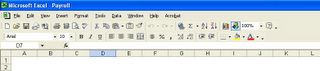
Tool_Bar_Final
Have a blessed weekend.

Tool_Bar_Original

The problem with this presentation is that the icons in both toolbars are not fully displayed. In this case, it would have been difficult for you to know all the shortcuts you could use (with the icons) since you can't see them. To make full use of the icons given in these 2 toolbars, you need to separate them. Here is how:
1) Move your mouse cursor along the icons in the toolbars from the left to the right. As you move to the right, the cursor will become a shape with 4 arrows pointing in 4 different directions.

Tool_Bar_Move
2) When the shape appears, click and hold onto the left mouse button and move the tool bar slight downward. The 2 toolbars will be presented in 2 rows and you would be able to see the full range of icons for the 2 toolbars.
3) Let go of the mouse button and you are done. You should be able to see your 2 toolbars presented as follows:

Tool_Bar_Final
Have a blessed weekend.
Thursday, January 05, 2006
What is the fastest way to do this?
Happy New Year to you. I wish you and your family a blessed 2006.
My apologies for not updating the blog for such a long time. The last 2 weeks was extremely busy for me as I rush for a number of my projects. I received a query and thought it would be good to share the answer with all of you. The question is as follows:
What is the fastest way to do this: check the cells for zero and delete the row if it is zero.
Solution
1) Highlight the list in the Excel Worksheet.
2) Go to Menu and select Edit, Find or use "Ctrl F" (shortcut key)
3) Type in the number "zero"
4) Click on the "Find ALL" button. Make sure that the option exact match is selected. This is to make sure that MS Excel does not return those cells with zero such as 10, 20, 30 , etc.
5.)Select the list by
5a) Go to the first item in the list.
5b) Hold on the shift key and click on the last item in the list.
5c) You have highlighted the entire list (See diagram below)
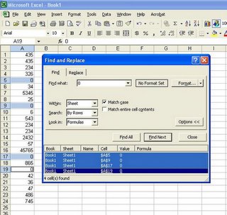
6) Close the find and replace dialog box.
7) Delete the rows using the following command. Edit >Delete and select entire row and click Ok.
The rows with zeros are deleted.
That's all for today. Drop me an email if this has been useful to you.
Cheers.
My apologies for not updating the blog for such a long time. The last 2 weeks was extremely busy for me as I rush for a number of my projects. I received a query and thought it would be good to share the answer with all of you. The question is as follows:
What is the fastest way to do this: check the cells for zero and delete the row if it is zero.
Solution
1) Highlight the list in the Excel Worksheet.
2) Go to Menu and select Edit, Find or use "Ctrl F" (shortcut key)
3) Type in the number "zero"
4) Click on the "Find ALL" button. Make sure that the option exact match is selected. This is to make sure that MS Excel does not return those cells with zero such as 10, 20, 30 , etc.
5.)Select the list by
5a) Go to the first item in the list.
5b) Hold on the shift key and click on the last item in the list.
5c) You have highlighted the entire list (See diagram below)
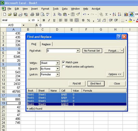
6) Close the find and replace dialog box.
7) Delete the rows using the following command. Edit >Delete and select entire row and click Ok.
The rows with zeros are deleted.
That's all for today. Drop me an email if this has been useful to you.
Cheers.
Friday, December 23, 2005
The Top Ten secrets of Excel
Hi all,
My apologies for not updating the blog for such a long time. I have been overwhelmed with work that I could not find the time to provide new information to you. It is quite coming up with topics out of the blue. As such, I appeal to you to send me some of your Exel-related problems and I will solve it FOC. The condition is that I could share it with others on the blog.
Last week, I have attend a live telecast called the "Learn 10 Secrets About Excel" You can view it online @ https://www118.livemeeting.com/cc/mseventsbmo/viewReg or download the whole e-book at a cheaper.
My apologies for not updating the blog for such a long time. I have been overwhelmed with work that I could not find the time to provide new information to you. It is quite coming up with topics out of the blue. As such, I appeal to you to send me some of your Exel-related problems and I will solve it FOC. The condition is that I could share it with others on the blog.
Last week, I have attend a live telecast called the "Learn 10 Secrets About Excel" You can view it online @ https://www118.livemeeting.com/cc/mseventsbmo/viewReg or download the whole e-book at a cheaper.
Saturday, December 17, 2005
A quick way to copy formula down hundreds of rows.
If you have 2 columns with 1000 rows each (say column A and B) and you created a formula in the first row (e.g. in column C). In most cases, you would have copied the formula throughout the 1000 rows by dragging the formula down. And one problem you faced is that you would take quite a while to drag to the 1000th row. In addition, you are likely to drag beyond the 1000 rows and have to back track.
Now, there is a simpler way. It just take 2 seconds to copy the formula down 1000 rows, or even 10000 rows. What you have to do is to move your mouse cursor to the bottom right corner of the formula cell in column C until a cross appears. Then double click on your left mouse button. Excel will make reference to the cells to the left of the formula cell (Column B in this case) and copy the formula all the way down to the last row (reference to column B). And you are done.
Enjoy your weekend.
Now, there is a simpler way. It just take 2 seconds to copy the formula down 1000 rows, or even 10000 rows. What you have to do is to move your mouse cursor to the bottom right corner of the formula cell in column C until a cross appears. Then double click on your left mouse button. Excel will make reference to the cells to the left of the formula cell (Column B in this case) and copy the formula all the way down to the last row (reference to column B). And you are done.
Enjoy your weekend.
Friday, December 16, 2005
The power of Pivot Table (Part VIII)
My apologies for not blogging for the past 2 days. I have to attend a conference on coporate planning and was busy preparing for my presentation for the conference. I was also trying to meet some project schedules.
I guess this should be the last posting on Pivot Table. There are too many things to cover on Pivot Table that I can spend 2 full days sharing with you all that I know. Having said that, I didn't want to bore you with more details until you have played around with those that I have posted in the last 2 weeks.
Do you know that Excel Pivot Table can give you the raw data that make up a particular result in one single step?
For example, if you are to double click on any one of the Sum of Amount cells, Excel will present the string of records that make up that number in another new worksheet. It will give you all the other details including fields that are not even presented in the pivot table. This is a wonderful function because it allows you to drill down to the most basic details. I don't think crystal report or Business Objects provide that. I may be wrong though.
I guess this should be the last posting on Pivot Table. There are too many things to cover on Pivot Table that I can spend 2 full days sharing with you all that I know. Having said that, I didn't want to bore you with more details until you have played around with those that I have posted in the last 2 weeks.
Do you know that Excel Pivot Table can give you the raw data that make up a particular result in one single step?
For example, if you are to double click on any one of the Sum of Amount cells, Excel will present the string of records that make up that number in another new worksheet. It will give you all the other details including fields that are not even presented in the pivot table. This is a wonderful function because it allows you to drill down to the most basic details. I don't think crystal report or Business Objects provide that. I may be wrong though.
Tuesday, December 13, 2005
The power of Pivot Table (Part VII)
Let's have something simple today. Now if you have a pivot table that shows two attributes on the left column of the pivot table, i.e. Customer Name followed by Promotion as per our pivot table we created in PART V. Do you know that you could hide the details such as those under promotion?
- What you need to do is to double click on a particular customer name and the promotion details are hidden.
- To unhide the details, double click on customer name again and the details under promotion appear.
Saturday, December 10, 2005
The power of Pivot Table (Part VI)
First, let us recap what we have covered so far.
1) We have learnt how to create a pivot table.
2) Format the results
3) Present the company sales results by customers, by promotion and by salesman.
I mentioned in point 3 that the sales results were company's results. What if you want to find out who are the key customers in a particular category or division? Here is how:
a) Move your mouse over the pivot table.
b) Click on the right mouse button and select wizard.
c) When you are brought back to Step 3 of 3 of the wizard, click on the layout button.
d) Notice on the top left hand corner that say page? Drag and drop the field call "division" into the page area.
e) Click Ok to get out of the layout dialog box and click finish to complete the wizard.
f) On the top left hand corner of the pivot table, you will see the field "division". With this, you can select the desired division and the data are filtered to show only the top selling customers by promotion by salesmen for the that division.
I hope I have amazed you with what Excel can do. Please come back if you want to discover more. Do come back if you are still not convinced about the power of Excel.
Have a blessed weekend.
1) We have learnt how to create a pivot table.
2) Format the results
3) Present the company sales results by customers, by promotion and by salesman.
I mentioned in point 3 that the sales results were company's results. What if you want to find out who are the key customers in a particular category or division? Here is how:
a) Move your mouse over the pivot table.
b) Click on the right mouse button and select wizard.
c) When you are brought back to Step 3 of 3 of the wizard, click on the layout button.
d) Notice on the top left hand corner that say page? Drag and drop the field call "division" into the page area.
e) Click Ok to get out of the layout dialog box and click finish to complete the wizard.
f) On the top left hand corner of the pivot table, you will see the field "division". With this, you can select the desired division and the data are filtered to show only the top selling customers by promotion by salesmen for the that division.
I hope I have amazed you with what Excel can do. Please come back if you want to discover more. Do come back if you are still not convinced about the power of Excel.
Have a blessed weekend.
Friday, December 09, 2005
The power of pivot table (Part V)
If you have followed through my recent blogs on The power of Pivot Table Part I to Part VI, you would have formatted the pivot table in a presentable format with the customers ranked by the total amount they have purchased from the company in descending order. The pivot table would have displayed which salesmen have sold products to the customers.
You may find that the above format is not sufficient for you to make decision on how you should classify the customers. You wonder whether the top customers are purchasing more of promotion items or normal items from you. Is pivot table able to do that? The answer is yes and here is how:
1) Move the mouse pointer over the pivot table.
2) Right click the mouse button.
3) A pop up menu will appear. Look for wizard and select it.
4) You are brought back to the step 3 of the pivot table wizard. Click on the layout button.
5) Now drag the field "promotion" from the list to the column area right below the customer name.
6) Click Ok and finished.
7) You should see the field "promotion" appearing on the left side of the "customer name"
8) Move the mouse button over the the right border of the row label as shown in this diagram.
9) Left click on the mouse button.
10) All the sub-total would be selected.
11) Highlight the sub-total with a color. For me, I would choose yellow.
Now you are able to make more informed business decisions with the additional dimension added.
Note: You can add as many dimensions to the column or row area. But remember that having more may not be better. Try not to micro analyse.
Take care and God Bless.
You may find that the above format is not sufficient for you to make decision on how you should classify the customers. You wonder whether the top customers are purchasing more of promotion items or normal items from you. Is pivot table able to do that? The answer is yes and here is how:
1) Move the mouse pointer over the pivot table.
2) Right click the mouse button.
3) A pop up menu will appear. Look for wizard and select it.
4) You are brought back to the step 3 of the pivot table wizard. Click on the layout button.
5) Now drag the field "promotion" from the list to the column area right below the customer name.
6) Click Ok and finished.
7) You should see the field "promotion" appearing on the left side of the "customer name"
8) Move the mouse button over the the right border of the row label as shown in this diagram.

9) Left click on the mouse button.
10) All the sub-total would be selected.
11) Highlight the sub-total with a color. For me, I would choose yellow.
Now you are able to make more informed business decisions with the additional dimension added.
Note: You can add as many dimensions to the column or row area. But remember that having more may not be better. Try not to micro analyse.
Take care and God Bless.
Wednesday, December 07, 2005
Back to The power of Pivot Table (Part IV)
Now that you have formated the results (Sum of Amount) for the pivot table, you might want to know that you could also rearrange the customers within the pivot table by ascending or decending alphabetical orders. That is not all. You can also arrange the customers list based on their purchases (ascending or decending order). What's more, you could even do a filter such that only the top x or bottom x number of customers are displayed in the pivot table.
Interested to find out how? Read on.
1) Double click on the grey box/button on the top left corner of the pivot table with the label "Customer Name"
2) A dialog box called Pivot Table Field wil appear. Click on the Advanced button.
3) Another Dialog box called PivotTable Field Advanced Options will appear.
4) Under the AutoSort Option, you can select Manual (Arranging the customer based on your own preference), ascending or descending order.
5) If you click on ascending or descending order, you would be able to choose the sorting preference, By customer name or by Sum of Amount (Purchases)
6) You can activate the Top 10 Auto Show by selecting the "on" option. Click on the drop down box and choose bottom if you decided to show the bottom x results in the pivot table. X is determined by the box next to the top/bottom selection.
7) If you have more than one result in the pivot table, you could select the field which the top or bottom x results should be based on.
8) Once you have made the relevant selection for the pivot table, click "ok" twice to return to the pivot table.
Task Completed.
God bless you with a wonderful day ahead.
If you want to learn about pivot table hands-on and are in Singapore on 12 and 19 Dec, you may want to consider signing up for my course. It will benefit those who are interested in business intelligence. Click here for more details.
Interested to find out how? Read on.
1) Double click on the grey box/button on the top left corner of the pivot table with the label "Customer Name"
2) A dialog box called Pivot Table Field wil appear. Click on the Advanced button.
3) Another Dialog box called PivotTable Field Advanced Options will appear.
4) Under the AutoSort Option, you can select Manual (Arranging the customer based on your own preference), ascending or descending order.
5) If you click on ascending or descending order, you would be able to choose the sorting preference, By customer name or by Sum of Amount (Purchases)
6) You can activate the Top 10 Auto Show by selecting the "on" option. Click on the drop down box and choose bottom if you decided to show the bottom x results in the pivot table. X is determined by the box next to the top/bottom selection.
7) If you have more than one result in the pivot table, you could select the field which the top or bottom x results should be based on.
8) Once you have made the relevant selection for the pivot table, click "ok" twice to return to the pivot table.
Task Completed.
God bless you with a wonderful day ahead.
If you want to learn about pivot table hands-on and are in Singapore on 12 and 19 Dec, you may want to consider signing up for my course. It will benefit those who are interested in business intelligence. Click here for more details.
Tuesday, December 06, 2005
Take a break from our Pivot Table Tutorial
I was reading an article in a Sinapore newspaper which talks about using business intelligence and using the right tool to yield predictive data. It was a worldwide bank which has successfully cull their databases for information as they assess the likely response for their new credit card.
As I read it, I was thinking that small and medium business owners must be envious of the cash that big corporations have to purchase tools to extract this data (customers' profile) out of their systems. What these small and medium business owners don't know (and I hope that they are reading this), is that their have the tool right in their desktops. Which tool is more suitable and at NO incremental cost to them than using Excel. I expect some of them to be skeptical about what I said but I would challenge them to find out more. One such evidence I have provided is the current subject which I have been sharing with you on this blog, that is, the Excel Pivot table.
It is not only capable of pulling out data from an Excel Spreadsheet. In fact, I have used Excel to pull out data from huge databases and present reports without the need to learn another software tool. Excel is all I need. If you are a small and medium business owner, come back often to this blog and you will know that I am not lying.
It was mentioned that business intelligence requires technologist and business analyst. True and not true. As I was working for some of the mobile companies and even a Fortune 500 company, I was the one (a business analyst) that are pulling out the data from databases and systems. And throughout my job, the IT department did not really intervene. If you are a business analyst, you must also be equipped with the skill of to cull databases or the concept of doing it. This is because data quality is important and half of these technologists do not know which set of data to extract. You have to because it affects your analysis. As the saying goes, garbage in garbage out.
There is so much to share and I can write and write but I wouldn't want to overload you with too much. I am planning to commit some resources to start a page on this. Look out for it. I am still planning the site.
If you want to learn about pivot table hands-on and are in Singapore on 12 and 19 Dec, you may want to consider signing up for my course. It will benefit those who are interested in business intelligence. Click here for more details.
As I read it, I was thinking that small and medium business owners must be envious of the cash that big corporations have to purchase tools to extract this data (customers' profile) out of their systems. What these small and medium business owners don't know (and I hope that they are reading this), is that their have the tool right in their desktops. Which tool is more suitable and at NO incremental cost to them than using Excel. I expect some of them to be skeptical about what I said but I would challenge them to find out more. One such evidence I have provided is the current subject which I have been sharing with you on this blog, that is, the Excel Pivot table.
It is not only capable of pulling out data from an Excel Spreadsheet. In fact, I have used Excel to pull out data from huge databases and present reports without the need to learn another software tool. Excel is all I need. If you are a small and medium business owner, come back often to this blog and you will know that I am not lying.
It was mentioned that business intelligence requires technologist and business analyst. True and not true. As I was working for some of the mobile companies and even a Fortune 500 company, I was the one (a business analyst) that are pulling out the data from databases and systems. And throughout my job, the IT department did not really intervene. If you are a business analyst, you must also be equipped with the skill of to cull databases or the concept of doing it. This is because data quality is important and half of these technologists do not know which set of data to extract. You have to because it affects your analysis. As the saying goes, garbage in garbage out.
There is so much to share and I can write and write but I wouldn't want to overload you with too much. I am planning to commit some resources to start a page on this. Look out for it. I am still planning the site.
If you want to learn about pivot table hands-on and are in Singapore on 12 and 19 Dec, you may want to consider signing up for my course. It will benefit those who are interested in business intelligence. Click here for more details.
Monday, December 05, 2005
The power of Pivot Table (Part III) - Formating the pivot table
After creating the pivot table, it is important to format the results from the pivot into an easily viewable format. This is important for your readers as well as for your own data analysis. By having a well formatted pivot table allows you to see the data patterns more clearly.
For example, the "Amount" field can be formatted the same way as a cell. The more important consideration is to ensure that the format remains even if you re-arrange the rows(in this case "customer names") and columns(Slsman No). This is how it should be done. Double click on the label called (Sum of Amount - from last week example). A dialog box appears. Click on the number button and the familiar dialog box for cell formating appears. Select the desired format and click Ok twice to complete the formating. The formating will be preserved even if the pivot table fields are re-arranged.
If you want to learn about pivot table hands-on and are in Singapore on 12 and 19 Dec, you may want to consider signing up for my course. Click here for more details.
For example, the "Amount" field can be formatted the same way as a cell. The more important consideration is to ensure that the format remains even if you re-arrange the rows(in this case "customer names") and columns(Slsman No). This is how it should be done. Double click on the label called (Sum of Amount - from last week example). A dialog box appears. Click on the number button and the familiar dialog box for cell formating appears. Select the desired format and click Ok twice to complete the formating. The formating will be preserved even if the pivot table fields are re-arranged.
If you want to learn about pivot table hands-on and are in Singapore on 12 and 19 Dec, you may want to consider signing up for my course. Click here for more details.
Friday, December 02, 2005
The power of Pivot Table (Part II)
Not convinced by what I have shared yesterday? Read on. I will prove to you with examples. The only way you can be convinced is to let you experience the power of Excel Pivot Table. Here's what I will do. Over the next few sessions, I will share with you what you could do with Excel Pivot Table and you judge for yourself whether what I said is true.
1) Download the data file I have created for you.
2) Open up the file.
3) Go to menu, data and select "pivottable and pivotChart report"
4) In step 1 of 3 of the pivot table wizard, select the option "Microsoft Excel List or database" and for the kind of report you want to create, select "pivot table"
5) Click Next
6) In Step 2, highlight the entire data table
7) Click Next,
8) Click on the Layout button when you are at step 3 of the pivot table wizard.
9) Drag the label called "customer" on to the section of the table called row.
10) Do the same for "Slsman No" and "Amount". The layout should look like this.
11) Click ok to go back to step 3 of the wizard.
12) Click Finish. Remove all the pop up boxes.
13) You should see the layout as shown in this diagram.
1) Download the data file I have created for you.
2) Open up the file.
3) Go to menu, data and select "pivottable and pivotChart report"
4) In step 1 of 3 of the pivot table wizard, select the option "Microsoft Excel List or database" and for the kind of report you want to create, select "pivot table"
5) Click Next
6) In Step 2, highlight the entire data table
7) Click Next,
8) Click on the Layout button when you are at step 3 of the pivot table wizard.
9) Drag the label called "customer" on to the section of the table called row.
10) Do the same for "Slsman No" and "Amount". The layout should look like this.

11) Click ok to go back to step 3 of the wizard.
12) Click Finish. Remove all the pop up boxes.
13) You should see the layout as shown in this diagram.

The power of Pivot Table (Part I)
For the benefit of those who don't know what is pivot table and how it works, I will start from basic and progress gradually from simple to difficult.
What is pivot table and what it can do?
Pivot table is a tool that is provided in Microsoft Excel Application. It's purpose is to help you analyze the data you have. Pivot table in Microsoft Excel seems like a cheapo tool to many because it is just one of the features in Excel. What most people don't know is that it would have serve the needs of most data analysers. In fact, with the right experience, Microsoft Excel pivot table would have diminished the value of the crystal reports based on the price paid. Not only crystal report, but it can be a strong competitor for business objects, inpromptu and other reporting tools. I have used these other tools listed and I still fall in love with Microsoft Excel Pivot Table. It is easy to use and the amount time you need to learn how to use pivot table is much less than those reporting tools listed. What more, Microsoft Excel is a tool that is familiar to you and most probably, you have it on your computer.
PS: I am conducting an Excel Workshop on the 12 and 19 Dec. If you are in Singapore during this 2 dates, yoiu might want to consider attending the course. Click here for more details
What is pivot table and what it can do?
Pivot table is a tool that is provided in Microsoft Excel Application. It's purpose is to help you analyze the data you have. Pivot table in Microsoft Excel seems like a cheapo tool to many because it is just one of the features in Excel. What most people don't know is that it would have serve the needs of most data analysers. In fact, with the right experience, Microsoft Excel pivot table would have diminished the value of the crystal reports based on the price paid. Not only crystal report, but it can be a strong competitor for business objects, inpromptu and other reporting tools. I have used these other tools listed and I still fall in love with Microsoft Excel Pivot Table. It is easy to use and the amount time you need to learn how to use pivot table is much less than those reporting tools listed. What more, Microsoft Excel is a tool that is familiar to you and most probably, you have it on your computer.
PS: I am conducting an Excel Workshop on the 12 and 19 Dec. If you are in Singapore during this 2 dates, yoiu might want to consider attending the course. Click here for more details
Wednesday, November 30, 2005
The power of Pivot Table
I have spoken to many and am amazed that many Excel users are not aware of the existence of pivot table. For some, they have heard of it but have not used it before. To these 2 groups of people, I must say that they have not truly experience the power of Excel. In fact, my performance in data analysis improved by leaps and bounds after I learnt about Excel's pivot table.
For those who have used Excel Worksheet as a data source, you are one step ahead of these two groups. But you are only using 30% of Excel's pivot table capability. Those who are already using MS Query would have harness the true power of Excel pivot table. In fact, it would take about a day for me to cover every aspects of Excel's pivot table. In the next few days, I would share with you some of these functions so that you could appreciate what Excel pivot tables can do for you and how it could improve your data analysis capability.
For those who have used Excel Worksheet as a data source, you are one step ahead of these two groups. But you are only using 30% of Excel's pivot table capability. Those who are already using MS Query would have harness the true power of Excel pivot table. In fact, it would take about a day for me to cover every aspects of Excel's pivot table. In the next few days, I would share with you some of these functions so that you could appreciate what Excel pivot tables can do for you and how it could improve your data analysis capability.
Tuesday, November 29, 2005
Getting the list of unique records (Method 2)
I have recently discover another method to retrieve the unqiue list of items. And here it is:
Assuming that you have the same list as yesterday.
1) Sort the list so that all the same items are group together.
2) Input a header on top of the list. This is required for the sub-total function we are going to use in the next step.
3) Activate the subtotal by going to menu, data, sub-total
4) When the dialog box appears, set the following options
a) At each change in: list (Header)
b) Use function: Sum
c) Add Subtotal to: list
d) Select the option: Replce current total
e) Select the option: Summary below data (see diagram for details)
5) Click OK.
6) Click on the button 2 located at the top left hand corner. The list would be compressed as shown in this diagram.
7) use the Goto Special function to extract the unique list to another excel worksheet.
8) Use the Replace function to remove the " total"
9) The list is extracted.
I might not be able to share more excel application with you on a daily basis from tomorrow till 12 Dec. This is because I might be tied up with the preparation of my Excel course which I am conducting on 12 Dec and 19 Dec (1.5 days in total). This is an inhouse course I am conducting for my client. As there are still some places left, my client has agreed to allow me to offer this course to you if you are interested. Of course, you must located in Singapore during this time. Drop me a comment if you are interested to find out more and I will furnish you with more details when it becomes available.
Assuming that you have the same list as yesterday.
What is a blog
Internet Marketing
Excel Formula
Adword Equaliser
Internet Marketing
Adword Equaliser
Excel Formula
Excel Formula
1) Sort the list so that all the same items are group together.
2) Input a header on top of the list. This is required for the sub-total function we are going to use in the next step.
3) Activate the subtotal by going to menu, data, sub-total
4) When the dialog box appears, set the following options
a) At each change in: list (Header)
b) Use function: Sum
c) Add Subtotal to: list
d) Select the option: Replce current total
e) Select the option: Summary below data (see diagram for details)

5) Click OK.
6) Click on the button 2 located at the top left hand corner. The list would be compressed as shown in this diagram.

7) use the Goto Special function to extract the unique list to another excel worksheet.
8) Use the Replace function to remove the " total"
9) The list is extracted.
I might not be able to share more excel application with you on a daily basis from tomorrow till 12 Dec. This is because I might be tied up with the preparation of my Excel course which I am conducting on 12 Dec and 19 Dec (1.5 days in total). This is an inhouse course I am conducting for my client. As there are still some places left, my client has agreed to allow me to offer this course to you if you are interested. Of course, you must located in Singapore during this time. Drop me a comment if you are interested to find out more and I will furnish you with more details when it becomes available.
Monday, November 28, 2005
Getting the list of unique records (Method 1)
Previously, we touched on the various methods to count the number of unique records listed in an excel worksheet. However, nothing was mentioned about producing the list of unique records using Excel. And I thought you might be interested to find out how. And here is one method you could use:
Assuming that the following product list is in column A starting in row 2.
What is a blog
Internet Marketing
Excel Formula
Adword Equaliser
Internet Marketing
Adword Equaliser
Excel Formula
Excel Formula
1) Sort the list so that all the same items are group together.
2) In cell A2, input the formula "=if (A2=A1,1,0)".
3) This formula will check to see if the cell A2 is the same as A1. If they are the same, the number 1 will appear. If they are different, the number 0 will appear. Since we have grouped the same items together, the 1 will appear if item appears the second or third time in the list. For example:
Assuming that the following product list is in column A starting in row 2.
What is a blog
Internet Marketing
Excel Formula
Adword Equaliser
Internet Marketing
Adword Equaliser
Excel Formula
Excel Formula
1) Sort the list so that all the same items are group together.
2) In cell A2, input the formula "=if (A2=A1,1,0)".
3) This formula will check to see if the cell A2 is the same as A1. If they are the same, the number 1 will appear. If they are different, the number 0 will appear. Since we have grouped the same items together, the 1 will appear if item appears the second or third time in the list. For example:
Adword Equaliser 0
Adword Equaliser 1
Excel Formula 0
Excel Formula 1
Excel Formula 1
Internet Marketing 0
Internet Marketing 1
What is a blog 0
4) Activate the autofilter function and filter using the criteria "0"
5) Once the duplicates are hidden, use the Goto Special function to extract the unique list to another excel worksheet.
Mission completed.
About Goto Special function
Press the F5 function key and then click on the Special button. Select the option "Visible Cells only" (see diagram). Click "OK". Only the visible cells are selected for now. Activate the copy function, go to another Excel worksheet, select a cell say A1 and activate the paste function.

Friday, November 25, 2005
Separate a string of values into different columns (Part III)
Spliting strings of values which are separated by a symbol is a breeze using the text to column function. What happens when you have a string without any separator, like those given below?
tops278484092828
name732180244063
baby276540921867
You can use the fixed width option instead of the delimited option in "Text to Column" function. For those who are using Excel 95 or 97 or evenExcel 2000, you might need to convert the font to one that is fixed width. This means that a "M" will occupy the same width as an "I". The font type I recommend is "Courier" or "Courier New".
Here are the steps:
1) Highlight the rows you want to parse.
2) Change the font to Courier.
3) Goto menu, Data, Text to Column
4) In step 1 of the wizard, select the option "fixed width". Click Next
5) Point the mouse pointer at the appropriate width and click the left mouse button once.
6) If you want to remove any of the preset separator, click the left mouse button at the appropriate black line or separator twice.
7) Once you have set the relevant width, click finish and the strings of value are separated into the respective columns.
Separate a string of values into different columns (Part II)
We found a way to split the values into the respective columns if they are separated by commas. What happens if they are separated not by commas but by the sign \ or ! or ~ ....... Is it possible then to separate them? The answer is yes. If we have a set of values which are separated by "" like those below , we can also split them up into the respective columns.
top 100 baby names\2784840\92828
This is how it should be done.
top 100 baby names\2784840\92828
baby names\732180\24406
baby\27654\09218
baby\27654\09218
This is how it should be done.
1) Highlight the rows you want to break up.
2) On the menu, select data, text to column.
3) In Step 1 of the wizard, make sure the option "delimited" is selected.
4) Instead of checking on the comma delimiters box as demonstrated yesterday, check on the box labelled others and input the sign "\" into the empty box that follows. Once you do that, the values are separated by black lines.
5) Click on finish and you are done.
Wednesday, November 23, 2005
Separate a string of values into different columns
Imagine you have a Comma Separated Values file (CSV in short). When you open the file, Excel fails to separate the values for you. No matter how many times you re-open the file, it remains as follows:
top 100 baby names,2784840,92828
baby names,732180,24406
baby,276540,9218
Are you going to separate them manually? On the above example, there are only 3 sets of values. What if there are 100 rows, 200 rows or more.
In Lotus 1-2-3, the function to separate the values is called parsing. In Excel, you can do the same through the function called "Text to Column".
1) Highlight the rows you want to break up.
2) On the menu, select data, text to column.
3) In Step 1 of the wizard, make sure the option "delimited" is selected. Click next.
4) Check on the comma delimiters box. Once you do that, the values are separated by black lines.
5) Click on finish and you are done.
The values are now separated into the respective columns.
top 100 baby names,2784840,92828
baby names,732180,24406
baby,276540,9218
Are you going to separate them manually? On the above example, there are only 3 sets of values. What if there are 100 rows, 200 rows or more.
In Lotus 1-2-3, the function to separate the values is called parsing. In Excel, you can do the same through the function called "Text to Column".
1) Highlight the rows you want to break up.
2) On the menu, select data, text to column.
3) In Step 1 of the wizard, make sure the option "delimited" is selected. Click next.
4) Check on the comma delimiters box. Once you do that, the values are separated by black lines.
5) Click on finish and you are done.
The values are now separated into the respective columns.
Tuesday, November 22, 2005
Calculating Working Days
Excel contains a function that helps you calculate the number of working days between 2 dates. It is called Networkdays. The function assumes a 5 days work week. To use the function, you need to activate an add-in called analysis toolpak. You can do this by going to the menu, tools, add-in and check on the box labelled "Analysis Toolpak". You may require Microsoft Office installation disk to activate the add-in.
The function also allows you to add in holidays such that they are excluded if these holidays fall on weekday and are within the period for the calculation.
The function also allows you to add in holidays such that they are excluded if these holidays fall on weekday and are within the period for the calculation.
Find out the number of unique products in the list (Second formula Explained)
We have covered the first formula last week, what about this second formula
=SUM(IF(FREQUENCY(IF(LEN(A1:A100)>0,MATCH(A1:A100,A1:A100,0),""),IF(LEN(A1:A100)>0,MATCH(A1:A100,A1:A100,0),""))>0,1))?
Before we share with you how the different functions are applied, do take note that the function starts with Sum(if and not sumif. There is a bracket in between the sum and the if. This denotes that it is a multi-conditional sum. To activate the formula, you need to use Ctrl + Shift + Enter together.
What are the conditions in the multi-conditions sum? Let's break them up and see what they meant
Click here for diagram
The formula Len(B1:B8)>0 is used to determine that the cell in the range is not a blank. If there is a character in the cell, then the length is at least 1 and it will return true as shown.
The formula shown in column D is developed to indicate the first row that the content shows up. For example, Internet marketing in row 6 returns a value of 3 because the phrase "internet marketing" shows up the very first time in Row 3.
In Column E, the formula frequency will calculate the number of times the number 1 shows up in the list in column D, followed by 2, 3, ..etc. Notice the simlarity in this formula with the complete formula =SUM(IF(FREQUENCY(IF(LEN(A1:A100)>0,MATCH(A1:A100,A1:A100,0),""),IF(LEN(A1:A100)>0,MATCH(A1:A100,A1:A100,0),""))>0,1)) In fact, the range D1:D8 as shown in the simplified formula is replaced by the formula show in prior column D. The replacement moves us closer to the complete formula. For clarity, the simlarities are highlighted in blue and green colour. Different colours are used to show that the range D1:D8 are replaced twice.
In the final part shown in column F, the formula =if(E5>0,1,0) is used to pass instruction to Excel to put in the number 1 in those rows in column F where the numbers showed up in column E is more than 0. By putting the conditional sum in the formula, we have completed the entire formula where the end result shown is the number of unique records in the list. Do remember to use Ctrl + Shift + Enter together to effect the formula.
=SUM(IF(FREQUENCY(IF(LEN(A1:A100)>0,MATCH(A1:A100,A1:A100,0),""),IF(LEN(A1:A100)>0,MATCH(A1:A100,A1:A100,0),""))>0,1))?
Before we share with you how the different functions are applied, do take note that the function starts with Sum(if and not sumif. There is a bracket in between the sum and the if. This denotes that it is a multi-conditional sum. To activate the formula, you need to use Ctrl + Shift + Enter together.
What are the conditions in the multi-conditions sum? Let's break them up and see what they meant
Click here for diagram

The formula Len(B1:B8)>0 is used to determine that the cell in the range is not a blank. If there is a character in the cell, then the length is at least 1 and it will return true as shown.
The formula shown in column D is developed to indicate the first row that the content shows up. For example, Internet marketing in row 6 returns a value of 3 because the phrase "internet marketing" shows up the very first time in Row 3.
In Column E, the formula frequency will calculate the number of times the number 1 shows up in the list in column D, followed by 2, 3, ..etc. Notice the simlarity in this formula with the complete formula =SUM(IF(FREQUENCY(IF(LEN(A1:A100)>0,MATCH(A1:A100,A1:A100,0),""),IF(LEN(A1:A100)>0,MATCH(A1:A100,A1:A100,0),""))>0,1)) In fact, the range D1:D8 as shown in the simplified formula is replaced by the formula show in prior column D. The replacement moves us closer to the complete formula. For clarity, the simlarities are highlighted in blue and green colour. Different colours are used to show that the range D1:D8 are replaced twice.
=SUM(IF(FREQUENCY(IF(LEN(A1:A100)>0,MATCH(A1:A100,A1:A100,0),""),IF(LEN(A1:A100)>0,MATCH(A1:A100,A1:A100,0),""))>0,1))
In the final part shown in column F, the formula =if(E5>0,1,0) is used to pass instruction to Excel to put in the number 1 in those rows in column F where the numbers showed up in column E is more than 0. By putting the conditional sum in the formula, we have completed the entire formula where the end result shown is the number of unique records in the list. Do remember to use Ctrl + Shift + Enter together to effect the formula.
Subscribe to:
Posts (Atom)